The Beta (β or beta coefficient) of a stock (or portfolio) is a measure of the (average) volatility (i.e. systematic risk) of its returns relative to the (average) volatility of the overall market returns (e.g. a benchmark index such as the S&P 500). β is used as a proxy for the systematic risk of a stock, and it can be used to measure how risky a stock is relative to the market risk. The β value of a stock can have the following interpretation:
You can use either of the three methods to calculate Beta (β) in excel, you will arrive to the same answer independent of the method. You can download my Excel file with all calculations and source data at the bottom of this page.
Levered beta (or equity beta) is the beta of a company inclusive of the effects from the capital structure. The beta that we calculated above is the Levered Beta.
Generally, a higher debt-to-equity ratio should cause the risk associated with a company’s equity shares to increase (all else being equal). The more debt a company has (and the higher the debt-to-equity ratio), the higher the risk of default (all else being equal).
Levered Beta = Unlevered Beta * [1 + (1 – Tax Rate) * (Debt / Equity)]
Unlevered beta, on the other hand, removes the effects from financial leverage to isolate the risk related to a company’s assets (i.e. pure business risk without any financial risk). For that reason, unlevered beta is often called “asset beta” because it measures the expected volatility of the underlying asset as if the company is completely financed by equity.
The levered beta of a firm is different than the unlevered beta as it changes in positive correlation with the share of debt of a company’s capital structure. Typically, a company’s unlevered beta can be calculated by taking the company’s reported levered beta from a financial database such as Bloomberg, Yahoo! Finance, Seeking Alpha or Google Finance and then applying the following formula:
Unlevered Beta = Levered Beta / [1 + (1 – Tax Rate) * (Debt / Equity)]
This page is advertising for FinancialTemplateStore.com. You can buy the Beta calculation template at their store by by clicking on the button below or click here.
Understanding beta is critical for investors seeking to evaluate asset risk and build optimal portfolios. Fortunately Excel makes calculating this important metric straightforward.
In this comprehensive guide, I’ll walk through everything you need to know to calculate beta in Excel like a pro. You’ll learn:
- What beta measures and why it matters
- Step-by-step instructions for calculating beta in Excel
- How to use Excel’s built-in functions for beta calculation
- Examples and sample templates for security and portfolio beta
- Techniques for analyzing and applying beta figures
- Limitations and pitfalls to watch out for
After reading this guide, you’ll be able to quickly find beta coefficients for stocks, ETFs, mutual funds, and any other security to make informed investment decisions. Let’s get started!
What Is Beta and Why Is It Important?
Beta measures the volatility of an asset compared to the overall market. It provides an estimate of how sensitive an investment’s returns are to macroeconomic movements and market risk.
Specifically, beta calculates the covariance between the asset’s historical returns and the benchmark’s (usually the S&P 500) divided by the variance of the benchmark’s returns
Stocks with a beta of 1 move in line with the broad market Betas greater than 1 indicate higher volatility than the market, while betas below 1 suggest more stability
As an investor, understanding beta helps you evaluate the risk-reward profile of assets and construct diversified portfolios. Securities with higher betas may generate excess returns but also experience bigger price swings.
By balancing high and low beta stocks and other asset classes, you can build optimal portfolios for your risk tolerance and goals. But first, you need to be able to accurately calculate beta.
Step-by-Step Instructions for Calculating Beta in Excel
Follow these steps to find beta in Excel for any security:
Step 1: Obtain Historical Price Data
To start, you need price history for the security you want to analyze and for a comparison benchmark.
For stocks, use the S&P 500 as the benchmark. For bonds, use an aggregate bond index. The minimum return history required is 24-36 months.
Step 2: Calculate Periodic Returns
Next, calculate the periodic returns for both the security and benchmark. The most common periods are daily, weekly, and monthly returns.
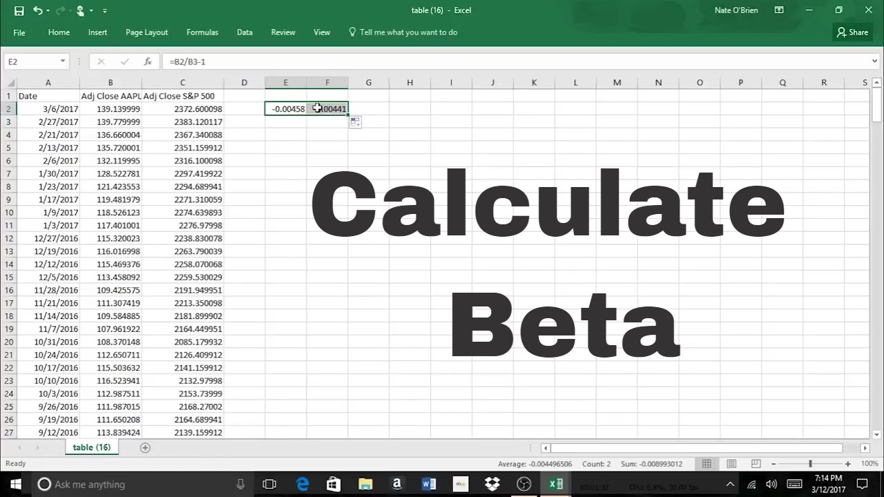
To find returns, use this formula:
=(Current Price/Previous Price)-1
Do this for the entire return history for both data sets.
Step 3: Find the Covariance
Use Excel’s COVAR function to calculate the covariance between the security’s returns and the benchmark’s returns:
=COVAR(range1,range2)
Range1 is the security’s returns and range2 is the benchmark’s returns.
Step 4: Determine Benchmark Variance
Use Excel’s VARP function to calculate the variance of the benchmark returns:
=VARP(range)
Where “range” is the benchmark return data.
Step 5: Calculate Beta
Finally, calculate beta by dividing the covariance result by the variance result:
Beta = Covariance / Variance
And that’s it – you now have the stock’s beta compared to the market!
Using Excel’s Built-in Functions
In addition to COVAR and VARP, you can also use:
- STDEV.P for benchmark volatility
- CORREL to analyze the return correlation
- SLOPE for regression-based beta
For example:
=SLOPE(security returns, benchmark returns)Gives you the regression beta based on linear regression analysis.
Experiment with different functions and methods to determine the optimal beta calculation for your needs.
Examples and Templates
Let’s walk through some beta calculation examples in Excel:
Stock Beta
You want to find the 3-year monthly beta for Apple (AAPL) compared to the S&P 500. You have 36 months of return history for both.
Use the COVAR and VARP functions to calculate:
=COVAR(AAPL_Returns, S&P_500_Returns) / VARP(S&P_500_Returns)Beta = 1.15This suggests AAPL has higher volatility than the overall market.
Portfolio Beta
Now you want to find the beta of a portfolio consisting of 50% AAPL, 30% SPY, and 20% bonds.
Use the weighted average betas of the components to derive the portfolio beta:
AAPL Beta = 1.15SPY Beta = 1Bond Beta = 0.5Portfolio Beta = (0.50 * 1.15) + (0.30 * 1) + (0.20 * 0.5) = 1.015The diversified portfolio has a beta very close to the market.
I’ve created an example template you can use to calculate beta for stocks, ETFs, and portfolios. Check it out!
Tips for Analyzing and Applying Beta Figures
Remember these tips when evaluating beta:
- Compare to market (S&P 500) beta of 1
- Look at betas for similar companies and industry averages
- Consider using adjusted betas (e.g. Blume, Vasicek)
- Account for different calculation periods producing different results
- Use beta for estimating relative, not absolute, risk
- Combine with other metrics like standard deviation and Sharpe ratios for robust analysis
Avoid over-reliance on beta as the singular indicator of risk. But appropriately applied, beta remains a useful tool for constructing diversified, risk-efficient portfolios.
Limitations and Pitfalls of Excel Beta
While easy to calculate in Excel, beta does have some limitations to be aware of:
- Assumes linear relationship between asset and market returns
- Vulnerable to estimation error with limited historical data
- May change significantly over time
- Doesn’t capture all risks like interest rates, geopolitics
- Difficult to apply reliably to less liquid assets
Use sound judgment when evaluating and applying beta figures in investment decisions. Weigh against other risk metrics and indicators to make informed decisions.
Now You’re a Beta Calculation Expert!
That wraps up this comprehensive guide to calculating beta in Excel. The key takeaways:
- Beta measures asset return sensitivity to market movements
- Excel makes finding beta easy using covariance and variance functions
- Apply beta to construct optimal portfolios and evaluate investments
- Combine beta with other metrics for robust risk analysis
Armed with these Excel skills, you can quickly find betas for any stock, fund, or portfolio to make informed investing decisions. Thanks for reading and happy beta calculating!
Step 4 – Calculate Beta – All 3 Methods (Regression, Slope & Variance/Covariance)
- Calculate the Variance of the benchmark using Excel’s VAR.P function
- Calculate the Covariance between the stock price returns and the benchmark price returns using Excel’s COVARIANCE.P function. Make sure you select the stock price returns as array1 in the function.
- Divide the Covariance by the Variance to calculate Beta. You could of course merge the two functions into a combined formula like this: =COVARIANCE.P(E7:E1263;F7:F1263)/VAR.P(F7:F1263)
Step 2 – Merge the stock and index data into a single table with a single “Date” column
You can use which return structure you like, e.g. logarithmic returns or “simple” returns. I have done both, please refer to the attached file for calculations and source data.
If you are not familiar with time series modeling, one would consider consider using logarithmic returns when doing time series modeling. Among other things due to that simple returns are not symmetric and are not additive over time. With other word, simple returns are not symmetric as positive and negative percentage returns of equal size do not cancel each other out. In addition, the sum of simple returns over multiple periods does not equal the total return across all sub-periods (from first to last period). Logarithmic returns, on the other hand, are symmetric and additive over time. For example, to summarize and calculate arithmetic mean makes sense when working with logarithmic returns. Please see the picture below for some examples.
How To Calculate Beta on Excel – Linear Regression & Slope Tool
How do you calculate the beta of a stock?
The beta, in the context of finance, is a measure of a stock’s volatility in the market. To calculate the slope of the beta, follow these steps: Organize your data: Create two columns, one for the stock’s returns and another for the market returns, over a specific period.
How do I calculate beta in Excel?
To calculate beta in Excel: Download historical security prices for the asset whose beta you want to measure. Download historical security prices for the comparison benchmark. Calculate the percent change period to period for both the asset and the benchmark. If using daily data, it’s each day; for weekly data, it’s each week, etc.
What does beta mean in Excel?
Beta measures how sensitive a firm’s stock price is to an index or benchmark. A beta greater than 1 indicates that the firm’s stock price is more volatile than the market. A beta less than 1 indicates that the firm’s stock price is less volatile than the market. Microsoft Excel serves as a tool to organize data and calculate beta. What Is Beta?
How do you calculate beta in a linear regression?
Divide the Covariance by the Variance to calculate Beta. You could of course merge the two functions into a combined formula like this: =COVARIANCE.P (E7:E1263;F7:F1263)/VAR.P (F7:F1263) Calculate the slope (Beta) of the linear regression line through data points (price returns) for the stock and the benchmark index.
