The tutorial shows how to use IFERROR in Excel to catch errors and replace them with a blank cell, another value or a custom message. You will learn how to use the IFERROR function with Vlookup and Index Match, and how it compares to IF ISERROR and IFNA.
“Give me the place to stand, and I shall move the earth,” Archimedes once said. “Give me a formula, and I shall make it return an error,” an Excel user would say. In this tutorial, we wont be looking at how to return errors in Excel, wed rather learn how to prevent them in order to keep your worksheets clean and your formulas transparent.
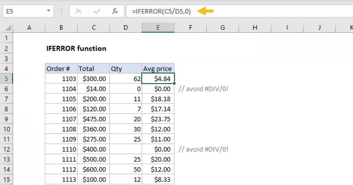
Working with formulas in Excel can sometimes lead to errors popping up all over the place. Errors like #DIV/0!, #N/A, #REF!, etc can make your spreadsheet look messy and confusing
This is where the IFERROR function comes in handy! IFERROR allows you to catch those errors and display something more readable instead It’s a simple way to clean up your Excel formulas,
In this beginner’s guide, I’ll explain everything you need to know about using IFERROR in Excel. We’ll cover:
- What is IFERROR and how does it work?
- Syntax and arguments
- Simple examples and common uses
- Advanced examples with other functions
- Pros and cons of IFERROR
- Alternatives to IFERROR
Let’s get started!
What is IFERROR in Excel?
The IFERROR function checks for errors in a formula. If there are no errors, it returns the result of the formula. But if there is an error, it returns a value you specify instead.
So in plain English, IFERROR works like this:
- Check for errors in this formula
- If there are errors, return this value instead
- If no errors, return the result of the formula
It’s an elegant way to handle errors and display something more readable in their place. No more ugly #DIV/0! or #N/A errors.
Syntax and Arguments
The syntax for IFERROR is simple:
=IFERROR(value, value_if_error)It accepts two required arguments:
-
Value – The formula or cell reference you want to check for errors.
-
Value_if_error – The value you want to return if there is an error.
Some examples of what you can use for value_if_error:
- Empty string (“”) for blank cells
- Custom error message like “No data”
- Number or string value
- Different formula or cell reference
Now let’s look at some simple examples of IFERROR in action.
Basic Examples of IFERROR
Here are a couple straightforward examples to show how IFERROR works.
1. Return a Blank Cell on Errors
=IFERROR(A2/B2,"")This checks A2/B2 for errors. If there are none, it returns the result. If there is an error like #DIV/0!, it returns a blank cell instead.
2. Display Custom Error Message
=IFERROR(A2/B2,"No data")Same check on A2/B2, but this time returning a custom message if there’s an error.
Very simple, but IFERROR becomes more powerful when combined with other functions.
Using IFERROR with Other Excel Functions
IFERROR really shines when you use it to handle errors from other functions like VLOOKUP, MATCH, INDEX, etc.
Here are some common examples:
1. IFERROR with VLOOKUP
VLOOKUP often returns #N/A errors when no match is found. Use IFERROR to catch those and display a message:
=IFERROR(VLOOKUP(A2,C2:D10,2,FALSE),"Not found") Now instead of #N/A errors, you get “Not found” for unmatched lookups. Much clearer!
2. IFERROR with Nested Formulas
You can nest IFERROR functions to perform sequential calculations:
=IFERROR(XLOOKUP(A2,Sheet1!A:B,2,0),IFERROR(VLOOKUP(A2,Sheet2!A:B,2,0),"Not found"))This tries XLOOKUP first, then VLOOKUP, returning “Not found” only if both produce errors.
3. IFERROR with Array Formulas
IFERROR works with array formulas too. It will return an array of values/errors:
=IFERROR(A2:A10/B2:B10,"")Any errors in the array formula will be replaced with blank cells.
As you can see, IFERROR is versatile and can be used in many different ways.
Pros and Cons of the IFERROR Function
Like any Excel function, IFERROR has both advantages and disadvantages:
Pros:
- Simple way to handle errors
- Can display custom messages
- Works on all Excel error types
- Available in all versions of Excel 2007+
Cons:
- Not as flexible as nested IF statements
- Can mask errors you actually want to see
- Requires two arguments instead of one like ISERROR
Next let’s look at some alternatives to IFERROR.
Alternatives to IFERROR in Excel
While IFERROR is the most common way to handle errors, there are a few other options:
-
IF and ISERROR – The old way to catch errors before IFERROR existed. More complex but more flexible.
-
IFNA – Only catches #N/A errors, not all errors. Useful when you only want to handle one error type.
-
TRY – New in Excel 2016, this works like exception handling in other languages. Lets you run code “try” a formula and “catch” any errors.
So IFERROR isn’t your only choice. But it strikes a good balance of simplicity and utility for most users.
Now you have a solid grasp of how to use IFERROR in Excel!
To quickly recap:
- IFERROR checks for errors in a formula
- If errors exist, it returns a value you specify
- If no errors, it returns the formula result
- Great for handling errors from VLOOKUP, MATCH, nested formulas, etc.
While not perfect, IFERROR is a quick and easy way to clean up spreadsheet errors. Use it to display custom messages instead of confusing error values.
Nested IFERROR functions to do sequential Vlookups in Excel
In situations when you need to perform multiple Vlookups based on whether the previous Vlookup succeeded or failed, you can nest two or more IFERROR functions one into another.
Supposing you have a number of sales reports from regional branches of your company, and you want to get an amount for a certain order ID. With A2 as the lookup value in the current sheet, and A2:B5 as the lookup range in 3 lookup sheets (Report 1, Report 2 and Report 3), the formula goes as follows:
=IFERROR(VLOOKUP(A2,Report 1!A2:B5,2,0),IFERROR(VLOOKUP(A2,Report 2!A2:B5,2,0),IFERROR(VLOOKUP(A2,Report 3!A2:B5,2,0),"not found")))
The result will look something similar to this: 
For the detailed explanation of the formulas logic, please see How to do sequential Vlookups in Excel.
IFERROR vs. IF ISERROR
Now that you know how easy it is to use the IFERROR function in Excel, you may wonder why some people still lean towards using the IF ISERROR combination. Does it have any advantages compared to IFERROR? None. In the bad old days of Excel 2003 and lower when IFERROR did not exist, IF ISERROR was the only possible way to trap errors. In Excel 2007 and later, its just a bit more complex way to achieve the same result.
For instance, to catch Vlookup errors, you can use either of the below formulas.
In Excel 2007 – Excel 2016: IFERROR(VLOOKUP(…), “Not found”)
In all Excel versions: IF(ISERROR(VLOOKUP(…)), “Not found”, VLOOKUP(…))
Notice that in the IF ISERROR VLOOKUP formula, you have to Vlookup twice. In plain English, the formula can be read as follows: If Vlookup results in error, return “Not found”, otherwise output the Vlookup result.
And here is a real-life example of an Excel If Iserror Vlookup formula:
=IF(ISERROR(VLOOKUP(D2, A2:B5,2,FALSE)),"Not found", VLOOKUP(D2, A2:B5,2,FALSE )) 
For more information, please see Using ISERROR function in Excel.
Introduced with Excel 2013, IFNA is one more function to check a formula for errors. Its syntax is similar to that of IFERROR: IFNA(value, value_if_na)
In what way is IFNA different from IFERROR? The IFNA function catches only #N/A errors while IFERROR handles all error types.
In which situations you may want to use IFNA? When it is unwise to disguise all errors. For example, when working with important or sensitive data, you may want to be alerted about possible faults in your data set, and standard Excel error messages with the “#” symbol could be vivid visual indicators.
Lets see how you can make a formula that displays the “Not found” message instead of the N/A error, which appears when the lookup value is not present in the data set, but brings other Excel errors to your attention.
Supposing you want to pull Qty. from the lookup table to the summary table as shown in the screenshot below. Using the Excel Iferror Vlookup formula would produce an aesthetically pleasing result, which is technically incorrect because Lemons do exist in the lookup table: 
To catch #N/A but display the #DIV/0 error, use the IFNA function in Excel 2013 and Excel 2016:
=IFNA(VLOOKUP(F3,$A$3:$D$6,4,FALSE), "Not found")
Or, the IF ISNA combination in Excel 2010 and earlier versions:
=IF(ISNA(VLOOKUP(F3,$A$3:$D$6,4,FALSE)),"Not found", VLOOKUP(F3,$A$3:$D$6,4,FALSE))
The syntax of the IFNA VLOOKUP and IF ISNA VLOOKUP formulas are similar to that of IFERROR VLOOKUP and IF ISERROR VLOOKUP discussed earlier.
As shown in the screenshot below, the Ifna Vlookup formula returns “Not found” only for the item that is not present in the lookup table (Peaches). For Lemons, it shows #DIV/0! indicating that our lookup table contains a divide by zero error: 
For more details, please see Using IFNA function in Excel.
How To Use The IFERROR Function In Excel – The Easy Way!
What is iferror function in Excel?
The IFERROR function in Excel is designed to trap and manage errors in formulas and calculations. More specifically, IFERROR checks a formula, and if it evaluates to an error, returns another value you specify; otherwise, returns the result of the formula. The syntax of the Excel IFERROR function is as follows: Where:
What is if error in Excel?
The IFERROR function in Excel handles all error types including #DIV/0!, #N/A, #NAME?, #NULL!, #NUM!, #REF!, and #VALUE!. Depending on the contents of the value_if_error argument, IFERROR can replace errors with your custom text message, number, date or logical value, the result of another formula, or an empty string (blank cell).
What is the difference between IFNA and iferror in Excel?
The IFERROR function catches all errors, whereas the IFNA function specifically catches #N/A errors. If you only want to catch #N/A errors, use the IFNA function instead of the IFERROR function. In the above discussion, we have shown you how to use the IFERROR function for about seven possible errors in Excel.
What is the difference between iferror and iserror in Excel?
If it does, the IFERROR function forces something to happen, like displaying an error message or value specified by you. Or running another formula. This makes it insanely valuable to trap and handle errors in Excel formulas. The ISERROR function is similar, but at the same time very different.
