When analyzing data in Excel, you may often want to switch rows to columns or columns to rows to change the orientation of your data. This is called transposing, and it rotates data 90 degrees.
Transposing in Excel is easy once you know how to do it. In this comprehensive guide, I’ll walk through step-by-step how to transpose Excel data using the copy and paste transpose method, keyboard shortcuts, and the TRANSPOSE function.
By the end, you’ll be able to effortlessly transpose rows and columns in Excel to wrangle your data any way you need.
What is Transposing in Excel?
Transposing in Excel exchanges the rows and columns in a cell selection. Any data laid out horizontally in rows will be rotated 90 degrees to sit vertically in columns, and vice versa.
For example suppose you have a dataset like this
| Week 1 | Week 2 | Week 3 | Week 4 |
|
Step 1: Select blank cells
First select some blank cells. But make sure to select the same number of cells as the original set of cells, but in the other direction. For example, there are 8 cells here that are arranged vertically:
So, we need to select eight horizontal cells, like this:
This is where the new, transposed cells will end up.
Step 2: Type =TRANSPOSE(
With those blank cells still selected, type: =TRANSPOSE(
Excel will look similar to this:
Notice that the eight cells are still selected even though we have started typing a formula.
3 Ways to Transpose Excel Data (Rotate data from Vertical to Horizontal or Vice Versa)
How do I move data from columns to rows in Excel?
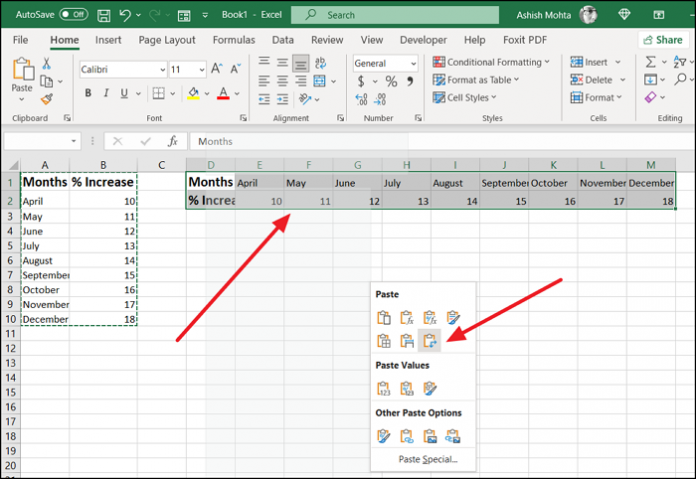
If you have a worksheet with data in columns that you need to rotate to rearrange it in rows, use the Transpose feature. With it, you can quickly switch data from columns to rows, or vice versa. For example, if your data looks like this, with Sales Regions in the column headings and Quarters along the left side:
How do I transpose a cell in Excel?
Click an empty cell and type in a reference and then the location of the first cell we want to transpose. I’m going to use my initials. In this case, I’ll use bcA2. In the next cell, below our first one, type in the same prefix and then the cell location to the right of the one we used in the previous step.
How to transpose data from rows to columns in Excel?
In Excel, you can transpose data from rows to columns. This is often used when you copy data from some other application and want to display it as column oriented. You can transpose rows from a single column, or transpose multiple column rows at once using Paste Special.
How do I transpose a row to a column in Google Sheets?
You can just as easily transpose rows to columns in Google Sheets. Select the range to transpose (A1:A8), right-click the selection, and choose Copy (or use CTRL + C ). Right-click the cell where you want to paste transposed data (B1), click Paste Special, and choose Transposed. As a result, values from Column A are now transposed in Row 1.
