How to Flip Columns in Excel: A Simple Guide for Reversing Data Order

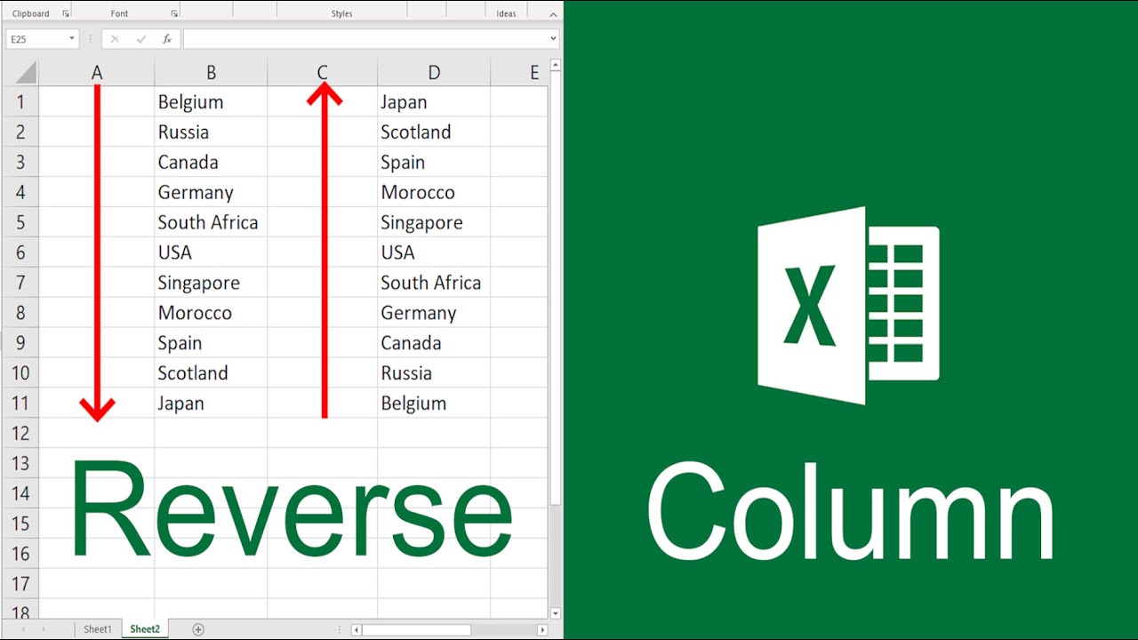
Flipping columns in Excel is a common task that allows you to quickly reverse the order of data. Whether you want to sort a column alphabetically in reverse or rearrange your data source, transposing columns can save you a lot of time.

In this comprehensive guide, I’ll walk you through the quickest and easiest ways to flip columns in Excel vertically. You’ll learn how to

• Flip columns using Sort
• Reverse column order with formulas
• Transpose data using VBA macros
• Flip columns while maintaining formatting and formulas

Let’s get started!

Why Flip Columns in Excel?

Here are some of the most common reasons you may need to flip columns in Excel

• Reverse alphabetical order – Flip columns sorted A-Z to Z-A
• Change data source layout – Rearrange the sequence of columns
• Analyze data differently – View columns in a different order for insights
• Present data variably – Flip orientation for reporting or visualization
• Fix imported data – Columns may import in the wrong order

Flipping columns allows you to resequence your data with just a few clicks. This can help uncover trends, visualize data better, and save you from tedious reordering tasks.

Flip a Column Using Excel Sort

The easiest way to reverse column order in Excel is by using the Sort feature.

Here are the steps to flip a column using Sort

1. Select the column you want to flip by clicking the column header.

2. Go to Data > Sort.

3. In the Sort dialog, select Sort Z to A. You can also sort by other options like dates, numbers, etc.

4. Hit OK.

This will instantly flip the selected column in reverse order. Sort is ideal when you have structured data that needs reversing, like dates, names, or values.

![Flip column using Excel Sort][]

However, for unstructured data, Sort won’t work as intended. We’ll look at other methods next.

How to Reverse Column Order in Excel Tables

To flip columns in a complete Excel table or dataset, we will need a helper column.

Follow these steps:

1. Insert a new helper column beside the data you want to flip.

2. In the helper column, enter a sequence of numbers starting from 1 in each cell. This numbering tip shows you how.

3. Select the helper column and sort the numbers Z to A. This will flip the adjacent data column too.

4. Once done, delete the helper column.![How to flip columns in Excel table][]

This method lets you quickly flip the order of any data column irrespective of its contents. The serial numbers act as the logic to reverse the sequence.

Flip Columns in Excel Using Formulas

Instead of Sort, you can also flip columns in Excel by using a simple INDEX formula: =INDEX(range, ROWS(range))

Where range is the data column you want to reverse.

Let’s see an example:

To flip Column A, the formula is =INDEX(A$2:A$6, ROWS(A$2:A$6)) ![Flip columns in Excel with formula][]

This formula fetches values from the bottom up in Column A and populates the new column B. ROWS acts as a decrementing counter and feeds the row numbers to INDEX in reverse order.

While this formula gets the job done, there are better programmatic ways using VBA.

How to Flip Columns in Excel with VBA Macro

For frequent column reversals, it’s best to use a VBA macro. The benefit is you can flip multiple columns in one go with a single click.

Here is the VBA code to flip columns in Excel: Sub FlipColumns()
Dim InputRange As Range Dim OutputRange As Range
Set InputRange = Application.InputBox(“Select columns to flip”, “Flip Columns”, , , , , , 8)
Set OutputRange = InputRange.Offset(, InputRange.Columns.Count)
For i = 1 To InputRange.Columns.Count
OutputRange.Cells(1).Offset(, i – 1).Value = InputRange.Cells(1).Offset(, InputRange.Columns.Count – i).Value
For j = 2 To InputRange.Cells(InputRange.Rows.Count, i).End(xlUp).Row
OutputRange.Cells(j).Offset(, i – 1).Value = InputRange.Cells(j, InputRange.Columns.Count – i + 1).Value
Next j Next i
End Sub

To use this VBA Macro:

1. Open VBE with Alt + F11 and insert a new module.
2. Paste the above code and press F5 to run.
3. When prompted select the column range to flip and click Ok.

This will instantly transpose the selected columns. You can modify the code further to add flexibility like flipping by a defined number of columns, etc.

Flip Columns While Keeping Formulas and Formatting

When you simply copy-paste or transpose columns, any formulas and formatting can get lost.

To flip columns and maintain all cell contents intact, you need a reliable flipping tool.

Ultimate Suite by Ablebits has a Flip feature that lets you vertically and horizontally flip data while retaining:

• All formulas and functions
• Cell formatting
• Charts and other objects
• Data validation

To use it to flip columns:

1. Select your data and go to Ablebits Data > Flip > Vertical Flip.

2. Choose options like Adjust references and Preserve formatting.

3. Hit the Flip button.![Flip columns while keeping formulas][]

The columns will be flipped seamlessly in a matter of seconds. You can be assured of accurate formulas and intact formatting.

Quickly Reverse Row Order in Excel

While we’ve focused on columns so far, you may also need to flip or reverse rows in your data. Here are a couple of quick ways to do this:

• Add a helper row with ascending numbers and sort the numbers Z to A.
• Use the same INDEX formula but with COLUMNS instead of ROWS.
• Transpose your data first, flip columns, transpose back.
• Use Ultimate Suite’s Horizontal Flip feature.![How to flip rows in Excel][]

Flipping rows horizontally will reverse the order of data from top to bottom. This can help pivot your data source or rearrange records.

Tips and Notes

Here are some additional pointers to keep in mind when flipping columns in Excel:

• Header rows will also be flipped, so exclude them if needed
• Double-check cell references in formulas after flipping
• Add a helper column on extreme right to avoid disrupting data
• Merge helper column approach with other methods like formulas
• If transposing entire sheet, consider converting to a Table first
• Always backup your data before flipping as a precaution

Flipping data order in Excel is easy once you know the right methods. Whether you want to reverse alphabetical order or rearrange your dataset, transposing columns can save you a lot of manual work.

The most flexible methods are using Sort with a helper column, INDEX/ROWS formula, and VBA macros. For error-proof results, a flipping tool like Ablebits Ultimate Suite is recommended.