Charts and other visual representations of data, such as financial, sales, or tax information, can be made by users in Microsoft Excel. Each Excel graph type allows users to integrate multiple graphical elements, including vertical lines. By clearly defining data information in Excel, learning to draw these vertical lines could increase your program knowledge and increase the accuracy of your graphs. This article explains why adding vertical lines to Excel graphs might be a good idea, how to add these lines to three different types of Excel graphs, and offers suggestions for streamlining the procedure.
How Can I Add a Vertical Line to an Excel Graph?
Improve the readability of your chart
Vertical lines and other graphic elements can help a chart stand out to readers and be easier to read. For instance, vertical lines can be used to make chart borders that delineate different data segments. Additionally, vertical lines may direct the reader’s attention downward and emphasize particular data on the chart. These straightforward design elements could increase chart readability by producing a more varied canvas and reducing eye fatigue or boredom.
Enhance chart structure and graphical design
Although borders and headers are included by default in Excel graphs, vertical lines may improve these structures. For instance, you could add more vertical lines to create thicker borders that set your data sets apart. On an Excel spreadsheet, vertical lines can also be used to connect related graphs and more effectively show how they are connected. Additionally, users have the option to increase the number of horizontal lines and make larger structural changes to their charts. This may make your chart easier to understand.
Use the efficiency of Excel formulas
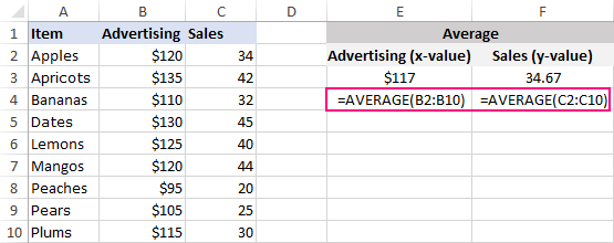
To make your vertical lines more fluid, you can enter different formulas into your Excel cells. For instance, you can enter vertical lines to chart graph averages and then add the average function. Input “=AVERAGE” and a parenthetical that includes the cell values. A completed average formula may read “=AVERAGE(B1,B2,B3,B4)” or similar. After that, depending on your needs for charting, you can use these values to create X or Y points. For instance, Y coordinate averages on a graph may be represented by vertical average lines. When drawing vertical lines, enter the cell name containing the average formula into the X or Y dialog window.
How to add vertical line to scatter plot
To highlight an important data point in a scatter chart and clearly define its position on the x-axis (or both x and y axes), you can create a vertical line for that specific data point like shown below: 
Naturally, since we don’t want to move the line every time the source data changes, we won’t “tie” a line to the x-axis. Our line will be dynamic and will automatically respond to any data changes.
What you must do in order to add a vertical line to an Excel scatter chart is as follows:
 Note. If youd like to draw a line at some existing data point, extract its x and y values as explained in this tip: Get x and y values for a specific data point in a scatter chart.
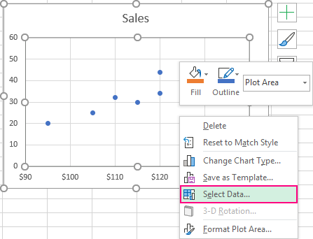
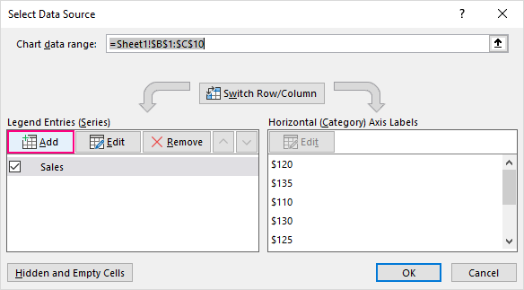
- Type a name for the vertical line series in the Series name box, such as Average.
- Choose the independentx-value for the relevant data point from the Series X value box. In this example, its E2 (Advertising average).
- Select the dependent value for the same data point in the Series Y value box. In our case, its F2 (Sales average).
- When finished, click OK twice to exist both dialogs.
Note. Be sure to delete the existing contents of the Series values boxes first – usually a one element array like ={1}. Otherwise, the selected x and/or y cell will be added to the existing array, which will lead to an error.
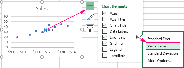
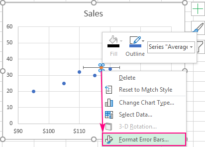
- If you want the vertical line to extend both upwards and downwards from the data point, set Direction to Both.
- For the vertical line to only point downward from the data point, change the direction to minus.
- To hide the horizontal error bars, set Percentage to 0.
- Setting Percentage to 100 and selecting the desired Direction will display a horizontal line in addition to the vertical line.
Done! A vertical line is plotted in your scatter graph. Depending on your settings in steps 8 and 9, it will look like one of these s: 
Actually, these are lines rather than columns, but I think either is acceptable. Looks great to me. What do you think? Let me know in the comments.
B) To create a line chart, select the New Data Range and highlight it. Your graph will have two horizontal lines and resemble the image below. Due to the fact that we have entered a value for every day, you can see the red horizontal line (labeled Vertical Lines). We wouldn’t have seen the line if we had only used a 12 on Tuesday and Thursday because those two data points weren’t adjacent, making it difficult for you to see and choose a line.
I want to express my gratitude to each and every one of you for supporting my blog and making it so popular once more. THANK YOU!.
This will give the lines the appearance that they run all the way up to the top of the vertical axis. Here is your final chart.
G) Alright, this completes the process for the simple dynamic vertical lines. To format an axis in Excel, right-click on the primary vertical axis and then select “Format Axis…”
One drawback is that you no longer have complete control over where the line will exactly cross the x-axis. You can compare the manual and embedded approaches in the table below. When using the manual method, the line can be drawn precisely on the tick mark between the data points for August and September, resulting in a neat alignment with the x-axis. The line is centered above the Sep label when using the embedded method, creating a marginally less seamless appearance.
I’ve developed one method for achieving this effect after doing some research and experimenting in Excel, which I’ll outline in this post (I’m sure there are others!). Don’t be put off by the lengthy setup process; it only requires one setup and can be quickly refreshed in subsequent iterations by shifting the location of the reference line. You can get the supplementary file by downloading Excel 2016, which I’m using.
The following chart illustrates what Dave describes. The data is units of output over time, with the final four months of the year being a forecast and the first nine months of the series being actual data. To distinguish between actual and forecast, the dotted line acts as a visual cue. The line was physically drawn on the graph using Shape Illustrator after being created in Excel. While this approach might work as a quick way to get the desired result, it isn’t the best for using the graph repeatedly, especially if the line’s location on the x-axis might change in subsequent iterations.
Losing the ability to alter the length of the line for labeling purposes is another drawback on the cosmetic front. I’ll use a horizontal bar chart I also made utilizing this technique to demonstrate this. Using the manual method, I can physically draw the line so that it rises above the x-axis line and is closely aligned with the text label “Target.” The embedded method leaves a space between the line and the label that describes it because the line remains below the x-axis line.
I currently have to draw them with the line drawing tool, which gets messy when moving the chart on a PPT slide. Dave asked: “Do you know of a trick for drawing vertical lines to delineate years (or actuals/historical vs forecast/future segments of the chart) It would be fantastic if there were a way to embed it in the data or format the chart in some way. ”.
FAQ
How do you get a vertical line on a graph in Excel?
- On the All Charts tab, select Combo.
- For the main data series, choose the Line chart type.
- Select Scatter with Straight Lines and the Secondary Axis checkbox for the Vertical Line data series.
- Click OK.
How do you make a vertical line graph?
Note: Before attempting to graph a vertical line that passes through a specific point, make that point. After that, simply draw a straight line through the point that is both up and down.
How do you add a line in a graph in Excel?
Choose the data series you want to add a line to from the chart, and then click the Chart Design tab. For instance, when you click a line in a line chart, all the data markers for that series are selected. Click Add Chart Element, and then click Gridlines.
What is a vertical line in Excel called?
Gridlines are the horizontal and vertical lines that separate the cells in a spreadsheet on the screen. Unless the option is set in the spreadsheet’s layout options, gridlines usually do not print.