Excel PivotTables are incredibly useful for summarizing and analyzing data With just a few clicks, you can group, sort, count, total or average data stored in a table or range
But sometimes, the built-in calculations aren’t quite enough. Fortunately, Excel provides two easy ways to customize and extend PivotTable calculations
- Calculated fields – Formulas that operate on the sum of the underlying data in a PivotTable.
- Calculated items – Formulas that operate on individual records in the source data.
In this article, we’ll explore calculated fields and calculated items in depth. You’ll learn how to add, modify and remove calculations to take your PivotTable reporting to the next level!
Let’s start with an overview of calculated fields.
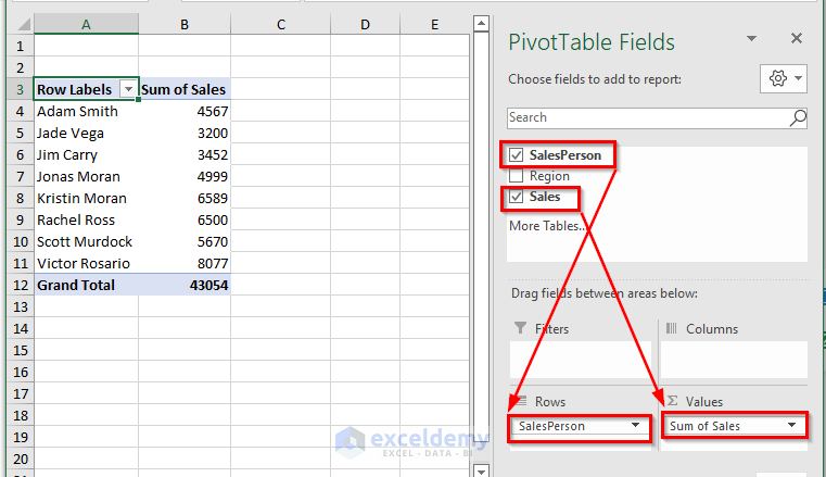
Calculated fields allow you to create new data fields in a pivot table that don’t exist in the source data. These new fields can be based on existing fields in the source data.
For example, suppose you have a PivotTable summing sales by region. You could make a calculated field called “Sales Commission” that shows 7% of the sales value
The result is a new field in the PivotTable that calculates dynamically based on the underlying data.
![PivotTable showing calculated field][]
A calculated field showing 7% sales commission
The best part is that calculated fields “travel” with the pivot table. If you refresh or rearrange the pivot table, the calculated values update automatically.
Calculated fields allow you to define custom summaries that aren’t available with regular pivot table value fields. With a simple formula, you can calculate sums, averages, percentages, max, min, standard deviations and much more.
Let’s look at how to add calculated fields to a PivotTable step-by-step.
How to Create a Calculated Field
-
Select any cell in the PivotTable. This will activate the PivotTable Tools menu.
-
Go to the Analyze tab > Calculations group > Fields, Items & Sets. Click “Calculated Field”. ![Go to Calculated Field][]
-
In the Insert Calculated Field dialog box: – Enter a name for the new field. – Enter the formula. Click fields or items to add them to the formula. – Click Add. ![Insert Calculated Field dialog][]
-
The new calculated field is added to the PivotTable! Formulas can use existing fields, expressions, numbers and functions. You can reference other PivotTable cells and ranges – but not worksheet cells/ranges.
That’s the basics of creating a calculated field. Next let’s look at some examples.
Calculated Field Examples
Here are a few common uses for calculated fields:
Percentage of Total
Show values as percentage of the overall total: =Sales / TOTAL(Sales)
Percentage Difference
Compare values to a base item: =Sales - BASE(Sales, "Apples")
Running Total
Cumulative sum in a specific order: =SUM(Sales) OVER (PREVIOUS([Region]))
Rank Smallest to Largest
Rank items from smallest to largest: =RANK(Sales, Sales, 1)
Index
Special calculated field for weighted percentages: =((Sales /GRANDTOTAL(Sales)) * (GRANDROW(Sales) / GRANDCOL(Sales))
These examples demonstrate the flexibility of calculated fields. You can perform quite advanced PivotTable calculations with simple formulas.
Next let’s go over a few key points when using calculated fields:
Name Calculated Fields Carefully
Use clear, descriptive names for calculated fields. This avoids confusion and errors if you have several calculations.
For example, name a field “Sales Commission” instead of just “Commission”.
Watch Out for Circular References
Avoid circular references where a calculated field refers to its own cell. This will result in a “Circular Reference” error.
For example, =Sales * 1.5 + SumSalesCommission will fail if SumSalesCommission refers to the current calculated field.
Limitations of Calculated Fields
There are a couple limitations to be aware of with calculated fields:
- Can’t reference cells outside the PivotTable.
- Calculation doesn’t happen row-by-row. The formula sees the pre-summarized values for each field.
- Grand totals don’t always calculate as expected.
We’ll talk more about handling grand totals next. Keep these limitations in mind as you work with calculated fields.
Handling Grand Totals
One issue with calculated fields is that grand totals don’t always calculate as expected.
For example, here is a PivotTable with sales commission calculated as 7% of sales:![PivotTable Grand Total issue][]
The grand total sums correctly for Sales. But the Sales Commission grand total is 7% of total sales, not the sum of commissions.
How can you avoid this issue? Here are 3 options:
1. Use GETPIVOTDATA to Reference Values
The GETPIVOTDATA function can pull specific PivotTable values into calculations.
For example, to sum commission total manually: =GETPIVOTDATA("Sales Commission", $A$3) + GETPIVOTDATA("Sales Commission", $A$4) + ...
This lets you control the calculation, avoiding the grand total issue.
2. Turn Off Grand Totals for Calculated Fields
Right click the pivot table and uncheck “Grand Totals for Rows” and/or “Grand Totals for Columns”.
This removes grand totals completely.
3. Filter Out All Records
Add a filter to the Row or Column area and filter out all records.
This will leave just the grand total row visible.
Next, let’s look at calculated items.
Introducing Calculated Items
In addition to calculated fields, PivotTables have “calculated items”.
Calculated items create custom calculations for specific pivot fields. They don’t create new fields, but rather new items within existing fields.
For example, you could make a calculated item that calculates a regional sales target:![Calculated items][]
Or a calculated item for sales excluding a specific product:![Calculated item example][]
Calculated items allow you to add custom items within fields, complementing calculated fields which make entirely new fields.
How to Insert a Calculated Item
The process for creating a calculated item is similar to a calculated field:
-
Click the field where you want to insert the calculated item.
-
Go to Analyze > Calculations > Calculated Item. ![Insert Calculated Item][]
-
Enter the Name and Formula. – Reference fields and items by enclosing them in double quotes. – Click Insert to add a field/item to the formula.
-
Click Add then OK to insert the calculated item.
And that’s it! With just a few clicks, you’ve customized the pivot field with a new calculated item.
Next, let’s go through some examples of calculated items.
Calculated Item Examples
Here are some common uses for pivot table calculated items:
Regional Sales Target
Calculate a target for each region by applying a growth percentage: =Sales * 1.10
Sales Excluding Product
Subtract sales for a particular product from total sales: =Sales - "Product A"[Sales]
Rolling Average Sales
Calculate a rolling 3 month average of sales for each region
Create List of Pivot Table Formulas
With a built-in pivot table command, you can quickly create a list of the calculated fields and calculated items in the selected pivot table.
| ▶ |
Note: NOTE: All pivot tables that share the same pivot cache will also share the same calculated fields and calculated items. |
To create a list of the pivot table formulas, follow the steps below:
- Select any cell in the pivot table.
- On the Ribbon, under the PivotTable Tools tab, click the Analyze tab (Options tab in some Excel versions).
- In the Calculations group, click Fields, Items & Sets
- Click List Formulas.
A new sheet is inserted in the workbook, with a list of the pivot tables calculated fields and a calculated items list.
- Calculated fields (if any), are listed first
- Calculated Items (if any), are listed second
- Solve Order is also shown, for calculated fields and calculated items
For details on how Solve Order works, go to the Pivot Table Calculated Items page.
Permanently Remove a Calculated Field
To permanently remove a calculated field, follow these steps to delete it:
- Select any cell in the pivot table.
- On the Ribbon, under the PivotTable Tools tab, click the Options tab (Analyze tab in Excel 2013).
- In the Tools group, click Formulas, and then click Calculated Field.
- From the Name drop down list, select the name of the calculated field you want to delete.
- Click Delete, and then click OK to close the dialog box.
How to add a calculated field to a pivot table
How to create a pivot table in Excel?
In Excel you can create a Pivot Table from any dataset, Pivot Table is useful when you need a new data point that can be obtained by using existing data points in the Pivot Table. Here you won’t need to go back and add it to the source data. Instead, by using a Calculated Field you can do this.
How do I add a calculated field to a pivot table?
1) Make sure you have a cell in the Pivot Table selected to activate the context-sensitive PivotTable Tools Analyze tab. In the Calculations Group, choose Fields, Items & Sets and select Calculated Field as shown. 2) Click on the drop-down arrow next to Name and select one of the calculated fields you created previously.
How do I add a formula to a pivot table?
Click in the Formula field. Enter a calculation using the fields in the list and/or custom values. You can also enter your own values in the formula. For example, you could find a monthly average by adding an existing field and then dividing by 12. Click OK. The new calculated field is automatically added to the PivotTable.
How to use pivot table analysis in Excel?
Select any cell in the Pivot Table to activate the PivotTable Analyze tab and click that. Expand the Fields, Items, & sets option in the Calculations group. Click “Calculated Field…” to open the “Insert calculated field” dialog box. Enter a name for the calculated field in the name box. So, you can type “Achievement %” in the name box.
