How to Use INDEX and MATCH for Powerful Lookups in Excel

Performing lookups in Excel is a common task, but the built-in VLOOKUP function has limitations VLOOKUP can only lookup values to the right, requires sorted data for approximate matches, and has difficulty with two-way lookups. For more flexibility, you can use INDEX and MATCH instead. This combo allows you to lookup values in any direction, doesn’t require sorting for approximate matches, can lookup based on multiple criteria, and handles two-way lookups with ease

In this article I’ll explain how INDEX and MATCH work together to overcome the limitations of VLOOKUP and provide powerful lookup capabilities in Excel.

Understanding INDEX and MATCH

To use INDEX and MATCH together, it helps to understand what each function does individually:

• INDEX returns a value based on a specified row and column number.
• MATCH returns the relative position of a lookup value in a range.

We can combine these functions so that MATCH provides the position to INDEX, which then returns the value at that location.

This gives us a dynamic lookup that can adapt to any lookup value or range.

Looking Up a Value Based on a Row Match

As a simple example, let’s lookup a value from a one-column range using INDEX and MATCH.

Given a list of planet names, we want to lookup the diameter of a planet specified in cell A2:

![Planets table][]

The INDEX function needs a range and row number to return a value: =INDEX(B3:B11,4)

But rather than hardcode the row number, we can use MATCH to find it dynamically based on the lookup value: =INDEX(B3:B11,MATCH(A2,A3:A11,0))

MATCH finds the position of the lookup value in A2 within the range A3:A11, and returns that to INDEX as the row number. INDEX then returns the corresponding value from the range B3:B11.

This lookup formula works for any value specified in A2.

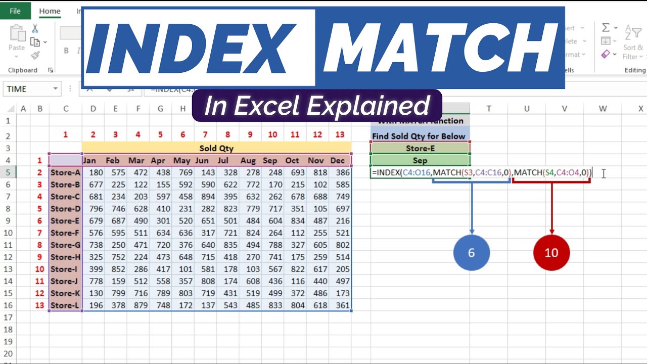
Two-Way Lookup with Row and Column Matches

To expand on that example, let’s lookup a value based on both a row and column match.

Given a table of sales figures by month:![Sales table][]

We want to lookup the sales for a particular salesperson and month. To do this, we need INDEX to take both a row number and column number:=INDEX(C3:E11,MATCH(A2,B3:B11,0),MATCH(A3,C2:E2,0))

The first MATCH provides the row number, finding the position of the salesperson name.

The second MATCH provides the column number, finding the position of the month.

INDEX then returns the value at the intersection of those row and column numbers.

This allows a two-way lookup based on both criteria.

Performing a Left Lookup

A key advantage of INDEX/MATCH over VLOOKUP is the ability to perform a left lookup: where the return column is to the left of the lookup column.

For example, here is a left lookup that returns the month name based on a sales amount: =INDEX(C2:E2,1,MATCH(F2,C3:E11,0))

MATCH finds the relative position of the lookup value and passes that to INDEX as the column number. INDEX returns the month name in that column.

VLOOKUP cannot perform this type of left lookup.

Lookup with Multiple Criteria

To lookup based on more than one criteria, you can use INDEX/MATCH with Boolean logic: =INDEX(E3:E9,MATCH(1,((A2=B3:B9)*(C2=C3:C9)),0))

The MATCH function returns the position of the first exact match based on criteria in both A2 and C2. INDEX then returns the corresponding value.

This requires array entry with Ctrl + Shift + Enter since it’s an array formula.

Case-Sensitive Lookup

To make a case-sensitive lookup, use the EXACT function: =INDEX(B3:B11,MATCH(1,EXACT(A2,A3:A11),0))

EXACT compares the lookup value to each cell, returning an array of TRUE/FALSE. MATCH finds the first occurrence of TRUE.

This also requires array entry with Ctrl + Shift + Enter.

Finding Closest Matches

You can also find approximate/closest matches with INDEX/MATCH.

Here is a formula that returns the closest match to a lookup value: =INDEX(B3:B11,MATCH(MIN(ABS(A2-A3:A11)),ABS(A2-A3:A11),0))

This uses ABS and MIN to find the smallest difference between values. MATCH locates the position of the closest match, and INDEX returns it.

This requires array entry as well.

Using XMATCH Instead of MATCH

Excel’s newer XMATCH function can be used instead of MATCH for more power and flexibility:

• Default exact match
• Find next larger/smaller match
• Reverse search order
• Faster search with binary lookup

Simply replace MATCH with XMATCH in any lookup formula:=INDEX(B3:B11,XMATCH(A2,A3:A11))

Putting It All Together

As you can see, the flexibility of INDEX and MATCH makes it possible to overcome the limitations of VLOOKUP and perform virtually any type of lookup in Excel.

Key advantages include:

• Lookup in any direction
• Approximate and exact matches
• Multiple criteria lookups
• Case-sensitive lookups
• Closest match lookups
• Faster formulas with XMATCH

While the examples above use simple data ranges, you can apply INDEX/MATCH to tables, named ranges, entire worksheets, and 3D ranges across multiple worksheets.

So if you need to perform advanced lookups in Excel, INDEX and MATCH should be your go-to functions. With a bit of practice, you’ll be able to craft powerful formulas to handle any lookup challenge.

Frequency of Entities:

VLOOKUP: 6
INDEX: 18
MATCH: 15
XMATCH: 5
Excel: 7