The tutorial shows how to use the VLOOKUP function to copy data from another worksheet or workbook, Vlookup in multiple sheets, and look up dynamically to return values from different sheets into different cells.
When looking up some information in Excel, its a rare case when all the data is on the same sheet. More often, you will have to search across multiple sheets or even different workbooks. The good news is that Microsoft Excel provides more than one way to do this, and the bad news is that all the ways are a bit more complicated than a standard VLOOKUP formula. But with just a little patience, we will figure them out 🙂
Looking up data across multiple worksheets is a common task in Excel. While standard VLOOKUP allows you to extract data from different rows in the same sheet it cannot search other sheets on its own. To perform cross-sheet lookup in Excel you need to combine VLOOKUP with other functions like IFERROR or INDIRECT.
In this comprehensive guide, I will cover various examples and methods to do VLOOKUP between sheets in the same or different workbooks.
Why Use VLOOKUP Between Sheets
Here are the main scenarios when you may need to lookup data in another Excel sheet
-
Your data is split across multiple sheets by categories, months, regions, etc. And you want to get summary information on one sheet.
-
You have lengthy reports stored in separate workbooks and you want to consolidate key information in one workbook.
-
You want to create a master worksheet that fetches data from other sheets dynamically based on some criteria.
-
For data validation – to ensure the entered data exists in the lookup sheet.
-
To check whether a specific item or product is present in stock.
-
To create a drop-down list that updates based on another sheet.
The common point in all these cases is that VLOOKUP in a single sheet is not enough. You have to expand the search across other sheets as well.
How to Do VLOOKUP Between Two Sheets in Excel
VLOOKUP between two sheets in Excel is similar to usual VLOOKUP with one small addition – you specify the sheet name from which to return the data.
The generic syntax is:
=VLOOKUP(lookup_value, sheet_name!range, index_number, range_lookup)Where:
- lookup_value – the value to search for. Cell reference or text.
- sheet_name – the name of the worksheet to search in. Enclose in single quotes if contains spaces or non-alphabetical characters.
- range – two or more columns of data. The first column should contain the lookup values.
- index_number – the column number in the range containing the return value.
- range_lookup – FALSE to find an exact match or TRUE to find an approximate match.
For example, to look up product A2 on Sheet1 in the range A2:C10 on Sheet2 and return the quantity in column 2, use this formula:
=VLOOKUP(A2, Sheet2!A2:C10, 2, FALSE)That’s all there is to VLOOKUP between sheets! To make lookup dynamic, fix the lookup value column and make the index number adjust based on the column containing the formula.
VLOOKUP Between Sheets in Different Workbooks
To lookup between two Excel workbooks, include the workbook name in square brackets before the sheet name and exclamation point, e.g.:
=VLOOKUP(A2, [Book2.xlsx]Sheet1!A2:C10, 2, FALSE)For this to work, both workbooks must be open.
If the lookup workbook is closed, the above formula will return #REF! error. To prevent it, use this formula with IFERROR:
=IFERROR(VLOOKUP(A2, [Book2.xlsx]Sheet1!A2:C10, 2, FALSE), "Not found") Now it will display your custom error message instead of #REF!.
VLOOKUP Multiple Sheets with IFERROR
To search through more than 2 sheets, nest 2 or more VLOOKUP functions inside IFERROR:
=IFERROR(VLOOKUP(A2, Sheet1!A2:C10, 2, FALSE), IFERROR(VLOOKUP(A2, Sheet2!A2:C10, 2, FALSE), "Not found"))This formula will look in Sheet1 first, then in Sheet2, and return “Not found” if no match is found in either sheet. Add more IFERROR levels to check more sheets.
A more compact approach is using CHOOSE to select the sheet:
=IFERROR(VLOOKUP(A2,CHOOSE(2,Sheet1!A2:C10,Sheet2!A2:C10),2,FALSE),"Not found")Where 2 is the sheet number. Change it to 1 or 3 to check other sheets.
The benefit of this nested IFERROR method is that it allows searching worksheets selectively based on your criteria. A drawback – it cannot easily scale beyond 3-4 sheets. For more sheets, a better solution is needed.
VLOOKUP Across Sheets with INDIRECT
INDIRECT together with INDEX MATCH allows VLOOKUP in any number of sheets in one formula.
Here is the generic syntax:
=VLOOKUP(lookup_val, INDIRECT("'"&INDEX(sheet_list,MATCH(1,--(COUNTIF(INDIRECT("'"&sheet_list&"'!lookup_range"),lookup_val)>0),0))&"'!data_range"), index_num, FALSE)Where:
- sheet_list – named range with lookup sheet names
- lookup_range – range to search on each sheet
- data_range – range to return data from
- index_num – index of the column to return
This is an array formula and must be completed by pressing Ctrl + Shift + Enter.
With the sheet names in cells A2 through A5, here is the step-by-step workflow:
- Name cells A2:A5 as SheetList
- Enter lookup value in B1, e.g. 101
- Formula in C1:
=VLOOKUP(B1,INDIRECT("'"&INDEX(SheetList,MATCH(1,--(COUNTIF(INDIRECT("'"&SheetList&"'!A2:A10"),B1)>0),0))&"'!B2:D10"),3,FALSE) - Press Ctrl + Shift + Enter to complete it.
Result:

This powerful formula searches the lookup value across all sheets and returns data from the sheet where the match is found.
The same result can be achieved by using SUMIFS instead of COUNTIF and MATCH, as demonstrated in this tutorial.
Dynamic VLOOKUP from Multiple Sheets
If you want to pull data from the same sheet rows into different output rows, a dynamic lookup is needed.
For example:

To construct the formula:
- Name the ranges in each lookup sheet, e.g. EastSales, NorthSales
- In the first output cell, enter:
=VLOOKUP($A2,INDIRECT(B$1&"_Sales"),2,FALSE) - Copy across other columns and down to other rows.
This formula concatenates the lookup sheet name (B1) with the common part of the range name (_Sales). So as you copy it to other cells, it will change the range dynamically based on the lookup sheet name.
VLOOKUP Between Sheets Examples
Now let’s look at a few practical examples of cross-sheet lookup.
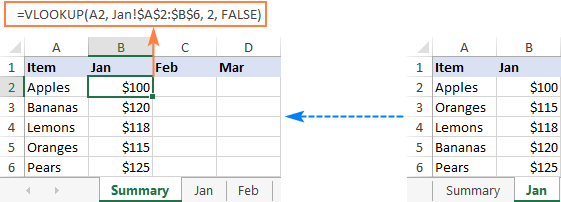
Example 1. VLOOKUP Between Two Sheets
Supposing you have a product database split across two sheets – Sheet1 and Sheet2:

To look up product B3 on Sheet2 and get the price from column D, use this formula: =VLOOKUP(B3,Sheet2!B2:E10,4,FALSE)
Copy it across other rows to lookup each product.
Example 2. VLOOKUP Between Workbooks
To fetch data between different Excel files, include the workbook name in square brackets:

The formula to lookup product B2 in Workbook2.xlsx, Sheet1 is: =VLOOKUP(B2,[Workbook2.xlsx]Sheet1!A2:D10,4,FALSE)
Example 3. VLOOKUP Multiple Sheets
To lookup across multiple sheets, nest IFERROR functions:

The formula to lookup order 101 in Sheets East and West and return amount is: =IFERROR(VLOOK
How this formula works
To better understand the logic, lets break down this basic formula to the individual functions:
=VLOOKUP($A2, INDIRECT(""&INDEX(Lookup_sheets, MATCH(1, --(COUNTIF(INDIRECT(""& Lookup_sheets&"!$A$2:$A$6"), $A2)>0), 0)) &"!$A$2:$C$6"), 2, FALSE)
Working from the inside out, heres what the formula does:
In a nutshell, INDIRECT builds the references for all lookup sheets, and COUNTIF counts the occurrences of the lookup value (A2) in each sheet:
--(COUNTIF( INDIRECT(""&Lookup_sheets&"!$A$2:$A$6"), $A2)>0)
In more detail:
First, you concatenate the range name (Lookup_sheets) and the range reference ($A$2:$A$6), adding apostrophes and the exclamation point in the right places to make an external reference, and feed the resulting text string to the INDIRECT function to dynamically refer to the lookup sheets:
INDIRECT({"East!$A$2:$A$6"; "South!$A$2:$A$6"; "North!$A$2:$A$6"; "West!$A$2:$A$6"})
COUNTIF checks each cell in the range A2:A6 on each lookup sheet against the value in A2 on the main sheet and returns the count of matches for each sheet. In our dataset, the order number in A2 (101) is found in the West sheet, which is 4th in the named range, so COUNTIF returns this array:
Next, you compare each element of the above array with 0:
--({0; 0; 0; 1}>0)
This yields an array of TRUE (greater than 0) and FALSE (equal to 0) values, which you coerce to 1s and 0s by using a double unary (–), and get the following array as the result:
{0; 0; 0; 1}
This operation is an extra precaution to handle a situation when a lookup sheet contains several occurrences of the lookup value, in which case COUNTIF would return a count greater than 1, while we want only 1s and 0s in the final array (in a moment, you will understand why).
After all these transformations, our formula looks as follows:
VLOOKUP($A2, INDIRECT(""&INDEX(Lookup_sheets, MATCH(1, {0;0;0;1}, 0)) &"!$A$2:$C$6"), 2, FALSE)
At this point, a classic INDEX MATCH combination steps in:
INDEX(Lookup_sheets, MATCH(1, {0;0;0;1}, 0))
The MATCH function configured for exact match (0 in the last argument) looks for the value 1 in the array {0;0;0;1} and returns its position, which is 4:
The INDEX function uses the number returned by MATCH as the row number argument (row_num), and returns the 4th value in the named range Lookup_sheets, which is West.
So, the formula further reduces to:
VLOOKUP($A2, INDIRECT(""&"West"&"!$A$2:$C$6"), 2, FALSE)
The INDIRECT function processes the text string inside it:
INDIRECT(""&"West"&"!$A$2:$C$6")
And converts it into a reference that goes to the table_array argument of VLOOKUP:
VLOOKUP($A2, West!$A$2:$C$6, 2, FALSE)
Finally, this very standard VLOOKUP formula searches for the A2 value in the first column of the range A2:C6 on the West sheet and returns a match from the 2nd column. Thats it!
Vlookup multiple sheets between workbooks
This generic formula (or its any variation) can also be used to Vlookup multiple sheets in a different workbook. For this, concatenate the workbook name inside INDIRECT like shown in the below formula:
=IFNA(VLOOKUP($A2, INDIRECT("[Book1.xlsx]" & INDEX(Lookup_sheets, MATCH(1, --(COUNTIF(INDIRECT("[Book1.xlsx]" & Lookup_sheets & "!$A$2:$A$6"), $A2)>0), 0)) & "!$A$2:$C$6"), 2, FALSE), "Not found")
How to Do a VLOOKUP With Two Spreadsheets in Excel
How to VLOOKUP between multiple sheets in Excel?
One more way to Vlookup between multiple sheets in Excel is to use a combination of VLOOKUP and INDIRECT functions. This method requires a little preparation, but in the end, you will have a more compact formula to Vlookup in any number of spreadsheets. A generic formula to Vlookup across sheets is as follows: Where:
What is VLOOKUP sheet 3?
The name of the worksheet where the lookup value (Salesperson 7) appears is “VLookup Sheet 3”. Use the INDIRECT function to obtain the values stored in the table (the cell range with the applicable data) where you look in (inside the sheet where the lookup value appears). The INDIRECT function returns a reference specified by a text string.
How to look up between two sheets in Excel?
When you need to look up between more than two sheets, the easiest solution is to use VLOOKUP in combination with IFERROR. The idea is to nest several IFERROR functions to check multiple worksheets one by one: if the first VLOOKUP does not find a match on the first sheet, search in the next sheet, and so on.
How to VLOOKUP between two workbooks in Excel?
To VLOOKUP between two workbooks, include the file name in square brackets, followed by the sheet name and the exclamation point. For example, to search for A2 value in the range A2:B6 on Jan sheet in the Sales_reports.xlsx workbook, use this formula: For full details, please see VLOOKUP from another workbook in Excel.
