needing to compare two data sets on a single Excel chart is a common challenge for analysts Visually juxtaposing the data makes it easier to spot trends and relationships between distinct data sets,
In this comprehensive guide, you’ll learn how to plot two data sets on the same chart in Excel using a combo chart.
Why Combine Two Data Sets on One Chart?
There are a few key reasons why you may want to graph two data sets together
-
Compare trends over the same time period – Viewing two data sets on a single timeline makes it easy to see if they follow similar or divergent patterns.
-
Contrast categories – A combo chart lets you quickly contrast values across categories for two distinct data sets.
-
Overlay correlations – Superimposing one data set on another allows you to check for potential correlations.
-
Conserve space – Plotting two sets together saves room compared to separate charts.
-
Simplify analysis – Having both data sets in one view makes analysis and insights more intuitive.
The ability to overlay two data sets in one Excel chart provides significant visualization benefits for drawing insights.
Step-by-Step Guide to Combining Data Sets
Follow these steps to elegantly plot two data series on the same chart in Excel:
-
Enter the data – Input each data set you want to plot into separate table areas. Format as an Excel table for easier charting.
-
Select the data – Highlight the table cells you want included for the first data series. Hold Ctrl and select the second table cells to combine.
-
Insert a combo chart – Go to the Insert tab and select the combo chart option. Choose the type that fits your data.
-
Edit the chart – Customize titles, legends, data labels, and axes to clearly distinguish the two data sets.
-
Format the data – Use contrasting colors and/or chart styles to differentiate the two data series.
-
Refine layout – Adjust column/row spacing so both data sets are clearly visible.
Let’s go through an example to see these steps in action.
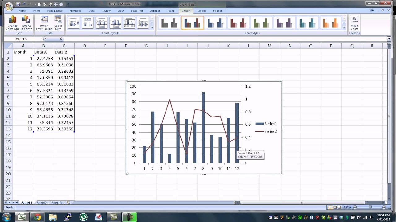
Example: Combining Revenue and Profit Data
Let’s say we want to compare a company’s revenue and profit over time on a single chart. We’ll combine these in a combo chart:
![Excel combo chart example][]
-
We input the revenue data in cells A2 to A7 formatted as an Excel table. Profit data goes in cells C2 to C7.
-
Select cells A2:A7 then Ctrl + select C2:C7 to choose both data ranges.
-
Go to Insert > Combo Chart and select the clustered column and line option.
-
Update the chart titles and legends to distinguish “Revenue” and “Profit”.
-
Apply contrasting colors and styles to the two data sets for easy visual separation.
-
Adjust row spacing on the y-axis to ensure both data sets are distinct.
The resulting combo chart clearly overlays the revenue and profit data in one compact view for easy analysis.
Key Combo Chart Settings
When working with combo charts, there are a few key settings to adjust:
- Data selection – Ensure you select the full data range for both series. The chart will only display the rows you highlight.
- Chart type – Select the type like clustered column and line that best fits your data. Consider the number of data series and data types.
- Legend – The legend distinguishes the data sets. Position it clearly.
- Data labels – Add labels to identify key data points. Make sure they don’t overlap.
- Colors – Use distinct colors and styles to differentiate data sets. This improves readability.
- Axis spacing – Adjust row and column spacing on the axes so all data is visible.
Tweaking these settings helps maximize clarity and understanding for the visualization.
Common Challenges and Solutions
When plotting two data series on one chart, a few common challenges can arise:
| Challenge | Solution |
|---|---|
| One data set dwarfs the other | Use secondary axis for smaller data set |
| Too many data points crowd the chart | Hide non-essential data points |
| Legend/labels cover up data | Reposition legend and reduce label text size |
| Hard to distinguish data sets | Apply contrasting colors and styles |
| Data sets overlap too much | Adjust axis minimum/maximum values |
A bit of reformatting and customization helps overcome these potential issues.
Best Practices for Overlay Charts
To create effective combo charts in Excel, follow these best practices:
- Ensure data sets are formatted consistently for accurate overlaying.
- Check that the chart type truly fits the nature of the data sets.
- Keep customization simple and tailored to focus on key insights.
- Use styles, colors, and labels judiciously to distinguish data sets.
- Adjust chart layout for ideal data visibility and comparison.
- Focus on consolidating data in one visual rather than intricate design.
The goal is an intuitive chart that provides an easy, accurate data comparison.
When Not to Use Combo Charts
Combo charts are not advisable in these cases:
- Unrelated data sets – Overlaying unrelated or incomparable data is confusing.
- Too many data series – More than 2-3 data sets clutter up the chart.
- Sparse data – Not enough data points make trends unclear.
- Incompatible ranges – Data set scales that are too different are hard to combine.
- Obscured insights – A simpler visual would bring out the insights better.
The key is to only combine data sets when the juxtaposition illuminates helpful insights.
Plotting two distinct data sets onto a single Excel chart provides a powerful visualization when done right. The key is choosing appropriate data sets, using a complementary chart type, customizing to focus on insights, and following combo chart best practices.
With this guide’s tips, you’ll be able to master overlaying data sets into compelling combo charts that extract hidden insights. So next time you need to graph two data series, use these techniques to create clear, effective charts that impress.
1 Answer 1 Sorted by:
If you want your plot to have data from both sets you can achieve it by
- Select the plot
- Goto “Design” tab and “Select Data”
- “Add” the new series and select data points in new series
And it will look like
But if you are worried about the spread of data in set 1 and set 2, and difficulty in pattern understanding, you can switch x & y and you can use secondary axis. This plot will look like
Hope you wanted either of this.
How to Add MULTIPLE Sets of Data to ONE GRAPH in Excel
Why is it important to show two sets of data in Excel?
It’s important to show two or more sets of data on one graph in Excel because it can help with: Below are steps you can use to help add two sets of data to a graph in Excel: 1. Enter data in the Excel spreadsheet you want on the graph To create a graph with data on it in Excel, the data has to be represented in the spreadsheet.
How do I plot multiple data sets on the same chart?
Often you may want to plot multiple data sets on the same chart in Excel, similar to the chart below: The following step-by-step example shows exactly how to do so. To create a scatter plot for Team A, highlight the cell range A2:B12, then click the Insert tab, then click the Scatter option within the Charts group:
Can you use multiple types of graphs in the same visual?
When you have two different data sets, it can be tempting to use multiple types of graphs in the same visual. When you use two sets of data, you are likely comparing them, so you can display both sets using the same methods for easy comparison.
