The XLOOKUP function in Microsoft Excel is a powerful search tool, allowing you to find particular values from a range of cells. It acts as the replacement for earlier lookup functions like VLOOKUP, eliminating many of their limitations.
As the name suggests, lookup functions like XLOOKUP pull matching data (exact matches, or the closest available match) from a dataset in Excel. If there’s more than one matching result, the first or last result in the set is returned, depending on the arguments used.
XLOOKUP acts as a custom search tool, flexible to the demands of different types of data in custom-built Excel spreadsheets. XLOOKUP is a relatively new function, only becoming available for Microsoft 365 users back in 2020. However, it’s quickly become one of the best Excel features for data analysis. If you’d like to start playing with data in Excel, have a go at our free 5-day data analytics short course to learn the basics.
The XLOOKUP function is an incredibly useful formula that allows you to look up data in Excel based on a search term. Introduced in Excel 365, it offers more flexibility and power than VLOOKUP
In this comprehensive guide, we’ll walk through how to use XLOOKUP in Excel step-by-step. You’ll learn how to perform vertical and horizontal lookups, return multiple values, handle errors, and more. Let’s get started!
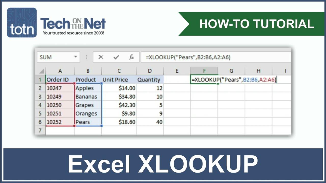
What is XLOOKUP?
XLOOKUP allows you to search for a lookup value in one column of a table or range and return a corresponding value from another column in the same row. This makes it perfect for tasks like
- Looking up an employee name based on their ID number
- Finding a product price from a product code
- Retrieving a customer’s phone number from their name
The key advantages of XLOOKUP over VLOOKUP are:
- Flexibility to look left or right for data
- Ability to return multiple values
- Additional options for exact, approximate and wildcard matches
- Better handling of errors
Now let’s walk through the syntax and arguments for this powerful function.
XLOOKUP Syntax and Arguments
Here is the syntax structure for XLOOKUP:
=XLOOKUP(lookup_value, lookup_array, return_array, [if_not_found], [match_mode], [search_mode])It has the following arguments:
- lookup_value – The value you want to search for. Required.
- lookup_array – The table or range to search in. Required.
- return_array – The table/range that contains the values to return. Required.
- if_not_found – Optional custom error to display if no match found.
- match_mode – Optional mode for exact, approximate or wildcard matches.
- search_mode – Optional mode for search direction and method.
Now let’s look at XLOOKUP examples that demonstrate how to use each argument.
Basic Exact Match XLOOKUP
Let’s start with a simple exact match XLOOKUP:
=XLOOKUP(B3,E2:E9,F2:F9)This looks in the lookup array E2:E9 for the lookup value in B3. When it finds a match, it returns the corresponding value from the return array F2:F9.
For example, if B3 contains “Banana”, it will return the price of 0.59 from column F.
By default, XLOOKUP does an exact match search from top to bottom. If no match is found, it returns #N/A.
Returning Multiple Values
A great feature of XLOOKUP is its ability to return multiple values from a single row.
For example:
=XLOOKUP(B5,C2:C9,C2:E9)This returns the first name, last name and email for the lookup ID in B5. The spill range contains multiple columns.
Looking Left with XLOOKUP
Unlike VLOOKUP, XLOOKUP can search for values in columns either to the left or right of the return column.
For example:
=XLOOKUP(G2,C2:C7,B2:B7)This looks for the salary value in column C, then returns the corresponding name from column B.
Handling Errors with XLOOKUP
To display a custom message if no match is found, use the if_not_found argument:
=XLOOKUP(B4,D2:D7,E2:E7,"No data") Now instead of #N/A, “No data” will display if the lookup value in B4 is not found.
Approximate and Wildcard Matching
To find the closest match or use wildcards, set the match_mode argument:
=XLOOKUP(B7,D2:D8,E2:E8,"",1)The 1 makes it return the next largest value when no exact match is found. Use -1 to get the next smallest.
You can also use wildcards like * and ? in the lookup value when match_mode is 2.
Performing Horizontal Lookups
While XLOOKUP is great for vertical lookups, you can also use it for horizontal ones:
=XLOOKUP(B3,C3:G3,C2:G2) This searches along row 3 for “Q1”, then returns the value at the intersection of that column and row 2.
Looking Up the Last Value
By default, XLOOKUP searches from top to bottom. To reverse the search order, set search_mode to -1:
=XLOOKUP(B8,C2:C9,D2:D9,,,,-1)Now instead of the first match, it will return the salary for the last instance of “John Smith”.
Performing a Binary Search
You can speed up XLOOKUP on sorted data by using search_mode 2 or -2 to perform a binary search.
Summary
- Lookup values on the left or right
- Return multiple columns
- Handle errors gracefully
- Search methods for fast performance
- Approximate and wildcard matching
With a bit of practice, you’ll be able to harness the full power of XLOOKUP to enhance your Excel data analysis.
Step 3: Determine the dataset using lookup_array and return_array
Once you’ve inserted the lookup value (your search value, or a cell reference containing it), you’ll need to identify your lookup_array and return_array cell ranges.
The lookup_array is the row or column that is likely to contain your search query (or nearest approximate result). The return_array is the row or column that you’d like to see returned as a result.
This could be a cell in another column on the same line (matching ID numbers to job roles in our example employee spreadsheet, for instance).
For our example, using =XLOOKUP(E3,A2:A10,D2:D10 means that the lookup_array used is the vertical cell range A2:A10, while the return_array is the vertical cell range D2:D10.
At this point, if you’re not interested in adding a custom error message, using a different search type (eg. approximate or wildcard matches), or changing the search value order, you can close your formula with a closing parenthesis. Otherwise, continue to add to your formula with optional arguments by following the steps below.
Step 1: Select an empty cell
To insert an XLOOKUP function in a new formula, start by opening an Excel spreadsheet containing your dataset and selecting an empty cell. Alternatively, open a new spreadsheet, leaving the spreadsheet containing your data minimized in another window.
Once the cell is selected, press the formula bar on the ribbon bar to begin to edit it.
The cell is active and ready for editing when the blinking cursor is visible on the ribbon bar. If this is the case, you’re ready to begin inserting a new XLOOKUP formula.
XLOOKUP in Excel Tutorial
How do I use XLOOKUP?
Use the XLOOKUP function to find things in a table or range by row. For example, look up the price of an automotive part by the part number, or find an employee name based on their employee ID.
How does XLOOKUP work?
Example 1 uses XLOOKUP to look up a country name in a range, and then return its telephone country code. It includes the lookup_value (cell F2), lookup_array (range B2:B11), and return_array (range D2:D11) arguments. It doesn’t include the match_mode argument, as XLOOKUP produces an exact match by default.
What is XLOOKUP function in Excel?
Example 5 uses a nested XLOOKUP function to perform both a vertical and horizontal match. It first looks for Gross Profit in column B, then looks for Qtr1 in the top row of the table (range C5:F5), and finally returns the value at the intersection of the two. This is similar to using the INDEX and MATCH functions together.
Does excel XLOOKUP work?
Yep, Excel XLOOKUP can do that too! You simply nest one function inside another: How this formula works: The formula is based on XLOOKUP’s ability to return an entire row or column. The inner function searches for its lookup value and returns a column or row of related data.
