How to Use the CHOOSE Function in Excel for Dynamic Flexibility

The CHOOSE function is an incredibly useful tool that provides dynamic flexibility within your Excel formulas. With CHOOSE, you can return different values from a pre-defined list based on an index number.

In this comprehensive guide, I’ll explain step-by-step how to use the CHOOSE function in Excel. You’ll learn how to create dynamic formulas that can adjust on the fly based on a changing index Let’s dive in!

What Does the CHOOSE Function Do in Excel?

The CHOOSE function allows you to specify a list of potential values as the function arguments. It will return whichever value corresponds to the index number provided.

For example, imagine you have a list of sales bonus percentages:

5%, 10%, 15%, 20%, 25%

You want to return one of those percentages based on a sales rep’s performance ranking

So if they are ranked 3, it should return 15%.

This is where CHOOSE comes in handy! It would look like:

=CHOOSE(3,5%,10%,15%,20%,25%)

By making the index dynamic, you can create flexible formulas that change output based on variable input.

How to Use the CHOOSE Formula in Excel

Using the CHOOSE function in Excel involves just 3 simple steps:

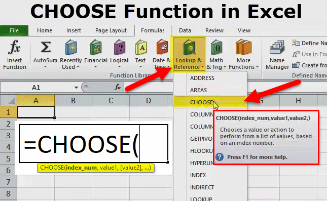
1. Insert the CHOOSE function. Select the cell where you want the returned value to appear. Type =CHOOSE( and the opening parenthesis.

2. Type your list of values. The first argument after “CHOOSE(” is the index number, but it’s often easier to first enter the list of potential values you want the formula to choose from. Separate each value by a comma.

3. Enter the index number. The index tells the function which value to return. Index 1 would return the first value, 2 the second value, and so on. Close the function with a final parenthesis.

And that’s it! Those three steps are all you need to use the CHOOSE function in Excel.

Let’s look at a more detailed example…

CHOOSE Function Example

Say you have a list of product prices based on quantity tier:

• 1-100 units = $5 each
• 101-500 units = $4 each
• 501+ units = $3 each

You want to create a formula where you can input the quantity purchased, and it will automatically return the right price per unit.

Here are the steps to use CHOOSE for this:

1. In cell B2, input the quantity purchased, like 250.

2. In C2, insert the CHOOSE function: =CHOOSE(

3. Add your list of potential values separated by commas:

=CHOOSE(B2,$5,$4,$3)

1. Close the function:

=CHOOSE(B2,$5,$4,$3)

Now cell C2 will display the price per unit based on the quantity in B2!

If you change the quantity, the price will automatically adjust thanks to the dynamic CHOOSE formula.

Tips for Using CHOOSE in Excel

When using the CHOOSE function, keep these tips in mind:

• Lists can contain numbers, text, cell references, or calculations.

• Nest CHOOSE within other functions like IF or VLOOKUP to extend functionality.

• Watch out for off-by-one errors – double check your index number corresponds to the intended return value.

• Error checking will display #VALUE! if index is <1 or > number of choices.

• Return blank cells instead of 0 with IF(ISNA(CHOOSE(),””,CHOOSE()) construction.

• Use CHOOSE to rank and assign letter grades, select colors dynamically, choose icons based on score, and more!

• For very long lists, reference cells instead of typing values directly to keep formulas clean.

• You can replicate CHOOSE with a nested IF statement but it’s messier and harder to maintain.

• When copying formulas, lock cell references with $ to prevent incorrect indices.

With creative use cases, the CHOOSE function provides endless possibilities for dynamic lookup formulas in Excel.

Common Uses for the CHOOSE Function

Beyond simple lists, what are some common real-world uses for the CHOOSE function in Excel?

Grading System

Use CHOOSE to assign letter grades based on numeric test scores:

=CHOOSE(CEILING(B2/10), "F","D","C","B","A")

Flooring the score divides it into 10 point buckets, rounding up. Then the grade text is returned.

Event Calendar

Pull event names into a calendar based on numeric date codes:

=CHOOSE(B2, "Birthday","Anniversary","Graduation","Holiday")

The date codes can be used as the index to return the matching event.

Commission Rates

Return commission percentages based on sales volume tier:

=CHOOSE(B2, 5%, 7%, 10%, 12%, 15%)

The higher the volume, the higher percentage they earn.

Dynamic Chart Colors

Color a chart series dynamically based on cell value:

=CHOOSE(B2, "Red","Orange","Yellow","Green","Blue")

The color text can be used in conditional formatting rules.

Patient Status

Classify patient status using categories:

=CHOOSE(CEILING(B2,0.5),"Critical","Serious","Fair","Good","Excellent")

Rounds the input score to assign a status category.

The possibilities are endless!

Troubleshooting Errors in CHOOSE Formulas

If you run into issues with the CHOOSE function returning errors or incorrect values, here are some troubleshooting tips:

• Double check the index number matches the intended return value position. Off-by-one mistakes are common.

• Make sure the index number is within the valid range for the number of arguments provided (1 to 256).

• Confirm cell references are locked properly when copying formulas to prevent shifting indices.

• Ensure all commas separating arguments are in place – missing commas will cause #VALUE errors.

• Try manually typing values instead of pointing to cell references to isolate the problem.

• Wrapping CHOOSE in IFERROR can display a custom message instead of #VALUE! errors.

• Start simple and add nested functions one at a time to identify where issues arise.

Following logical troubleshooting steps will help narrow down and resolve any issues with CHOOSE formulas.

Next Level: Creative Ways to Use CHOOSE in Excel

The CHOOSE function is ready to take your Excel skills to the next level. Here are some creative examples of advanced formulas with CHOOSE:

• Nested IF statements to check multiple criteria before selecting the CHOOSE index.

• LOOKUP functions to search categories and find the right index value.

• ROUND or PRODUCT to manipulate the index value into the needed range.

• MIN/MAX to constrain the index within upper and lower limits.

• MID or LEFT/RIGHT to extract just a portion of returned text values.

• CONCATENATE or & to combine chosen text items into full sentences.

• SUBSTITUTE to swap words within chosen text strings.

• Use CHOOSE to generate randomized data sets for analysis.

The key is imagining how CHOOSE can add flexibility within your existing formulas. The function really shines when you combine it creatively with other Excel tools.

Should You Use CHOOSE or a Nested IF?

A common question is when to use CHOOSE vs a nested IF statement. While both can provide similar output, here are some key differences:

• CHOOSE formulas are simpler and easier to read vs long nested IFs.

• CHOOSE allows you to easily maintain and add/remove options.

• Nested IFs allow more complex conditional logic before returning a value.

• CHOOSE has a limit of 256 arguments while nested IFs have no limit.

• CHOOSE avoids repetition of long IF statements checking the same criteria.

• CHOOSE avoids the extensive troubleshooting that comes with nested IFs.

In general, I would recommend CHOOSE for ease of use, flexibility, and maintenance. But nested IFs provide more custom control for complex logic requirements. Evaluate both to see which option makes more sense for your specific needs.

The CHOOSE function is an incredibly versatile tool that every Excel user should have in their formula toolkit. With the ability to return different values from a list based on an index number, CHOOSE provides dynamic flexibility to your models.

Now you have a clear, step-by-step understanding of how to use CHOOSE in Excel, from basic examples to advanced creative applications.

Put these skills into practice and CHOOSE will soon become your new go-to function for flexible lookup formulas. Your Excel skills will reach new