How to Unhide Columns in Google Sheets: A Complete Step-by-Step Guide

As a frequent Google Sheets user, you’ve likely hidden columns before to declutter your spreadsheet or emphasize certain data. But once hidden,you may eventually need to unhide columns again to access that data. Thankfully, it’s easy to unhide columns in Google Sheets on both desktop and mobile.

In this comprehensive guide, I’ll walk you through the quick steps to unhide columns in Google Sheets using simple clicks or taps. You’ll also learn how to unhide all columns at once, as well as tips for unhiding rows.

Follow these steps to effortlessly unhide columns and access your data again in Google Sheets on any device

Overview of Hidden Columns in Google Sheets

Before diving in. let’s look at some quick background on hidden columns in Google Sheets

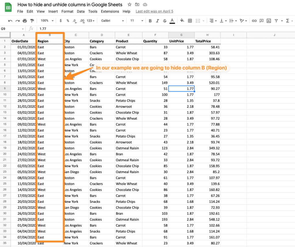
• Hidden with a click – Columns are hidden by clicking the column letter and selecting “Hide column” from the dropdown menu.

• Identified by missing letters – Hidden columns are indicated by missing column letters, like jumping from B to D.

• Located with arrows – Small grey arrows appear beside hidden column letters.

• Unhidden with a click – Clicking the arrow unhides the column again.

These basics on hidden columns set the stage for learning how to unhide them.

Unhide a Column Using the Arrows

The fastest way to unhide a column is by clicking the arrow icon next to a hidden column:

1. Open your Google Sheet on desktop or mobile.

2. Locate the hidden column by finding the missing column letters, like B to D.

3. Click or tap the small grey arrow next to the hidden column’s letter.

4. The column instantly reappears and is unhidden.

The small arrow provides a quick visual indicator and one-click method to unhide columns in Google Sheets.

Unhide Multiple Columns at Once

Rather than unhiding columns one by one, you can unhide multiple adjacent columns together:

1. Click the column letter on the left side of the hidden columns.

2. Scroll right and shift-click the column letter on the right side.

3. Right-click the selected columns.

4. Click “Unhide columns” from the context menu.

5. All columns within the selection will now be visible.

This speeds up the process when you have many neighboring columns to unhide.

Unhide All Columns in a Sheet

To instantly unhide every hidden column in a sheet:

1. Select all columns by clicking the column A letter.

2. Hold shift and click the last used column letter.

3. Right-click and choose “Unhide columns.”

4. All previously hidden columns will be made visible.

When you need to reset and see all columns again, this quick step does it in one click.

Unhide Columns on Mobile Devices

The process works the same whether you’re on a desktop or using the Google Sheets mobile app:

1. Open the sheet on your iPhone, Android, or tablet.

2. Tap the small grey arrow beside any hidden columns.

3. The column will be unhidden right away.

4. You can also long press a column and select “Unhide” to unhide.

Unhiding columns on mobile is just as easy as on desktop.

Unhide Columns Using Keyboard Shortcuts

For quick access without reaching for your mouse or touchscreen, Google Sheets offers keyboard shortcuts:

• Windows/Linux: Ctrl + Shift + E then S
• Mac: ⌘ + Shift + E then S
• Chromebook: Ctrl + Shift + E then S

After the keyboard command, hit S and all hidden columns are instantly shown.

Unhide Rows the Same Way

The steps to unhide rows are exactly the same:

• Click the arrow beside a hidden row number.

• Drag to select then right-click multiple rows and click “Unhide rows.”

• Use keyboard shortcuts Ctrl + Shift + E then R (Windows/Linux), ⌘ + Shift + E then R (Mac), or Ctrl + Shift + E then R (Chromebook).

Mastering unhiding columns transfers directly to unhiding rows!

Troubleshooting Hidden Columns

At times, you may run into problems while trying to unhide columns in Google Sheets:

• Arrows missing – If you don’t see arrows next to hidden columns, try restarting the browser or mobile app.

• Columns re-hide – Columns might re-hide on their own if you have “Hide columns” set in Conditional Formatting rules. Adjust or remove the rule.

• Can’t unhide – Make sure you’re the owner of the spreadsheet. Users without edit access can’t unhide columns.

• Wrong columns appear – If the wrong columns show, double check if data shifted. Columns may move if not locked in place.

Small issues like these are easily fixed once you know the cause behind columns disappearing again or showing incorrectly.

Customizing Hidden Columns

Beyond simply hiding and unhiding columns, Google Sheets provides additional options:

• Adjust column width – Widen or shrink visible portions of hidden columns.

• Change edit access – Set whether hidden columns are editable by other users.

• Protect data – Prevent unwanted editing of hidden columns.

• Link another sheet – Sync a hidden column to values from a different sheet.

Dig into these settings in column properties to tailor their functionality when hidden.

Functions to Try with Hidden Columns

Hidden columns open up useful possibilities using Google Sheets functions:

• =FILTER – Display a filtered data set excluding hidden columns.

• =SORT – Sort visible columns while keeping hidden data locked in position.

• =QUERY – Retrieve customized data from visible or hidden columns.

• =IMPORTDATA – Pull in live data from a published sheet but hide irrelevant columns.

The data in hidden columns remains accessible to work into creative formulas.

VLOOKUP with Hidden Columns

One common use case is using VLOOKUP to reference values present in a hidden column:

• Hide identifier columns – Use hidden columns for ID numbers or other internal identifiers.

• Retrieve data with VLOOKUP – The function reads hidden columns to find matching records.

• Show only relevant data – Visible columns display just the surfaced data without exposing identifiers.

This keeps sensitive IDs or keys hidden from view while VLOOKUP works behind the scenes with the full data set.

Common Reasons to Hide Columns

Hiding columns isn’t just about removing clutter. There are strategic reasons to hide columns in many situations:

• Hide irrelevant data – Focus attention on pertinent columns for the task at hand.

• Reduce scrolling – Decrease left-right scrolling on wide sheets by hiding unused columns.

• Anonymize data – Remove columns with personally identifiable information.

• Prevent edits – Hide columns that should stay locked to protect data integrity.

• Improve performance – Less data to render means faster load and refresh times.

Keep these use cases in mind as you consider when to hide columns – and when to unhide them again.

Alternatives to Hiding Columns

In some cases, you may want to consider options other than hiding:

• Filter views – Filter out unwanted data rows instead of entire columns.

• Separate sheets – Put less important columns on different sheets in the same workbook.

• Freeze columns – Lock columns in place so they don’t scroll off screen.

• Split data – Keep only high-value data in the sheet and move the rest to another data source.

Sometimes it makes more sense to keep columns visible but isolate or act on the data differently.

Best Practices for Organized Sheets

Use these best practices to keep your sheets well structured when hiding and unhiding columns:

• Label columns clearly so you know what’s hidden.

• Sort columns in logical order before hiding.

• Freeze columns in place so hiding others doesn’t shift data.

• Add comments explaining why columns are hidden.

• Be consistent on hiding columns so data stays aligned.

Building good habits around hiding columns saves headaches down the road!

Frequently Asked Questions about Unhiding Columns in Google Sheets

You probably have additional questions about unhiding columns in Google Sheets. Here are answers to some commonly asked questions:

How do I unhide every column at once?
Use the Select All columns keyboard shortcut Ctrl + A (Windows/Chromebook) or Command + A (Mac), then right click and choose Unhide Columns.

Where do hidden columns go in Google Sheets?
Hidden columns aren’t deleted – they’re simply not displayed. The data remains stored in the sheet. Unhiding