How to Search in Excel Like a Pro

Searching in Excel can be tricky if you don’t know the right techniques With large spreadsheets containing tons of data, trying to locate specific text, values or formulas can seem daunting

But it doesn’t have to be! With the right search skills, you can easily filter through thousands of rows and columns to find what you need.

In this comprehensive guide I’ll walk you through the various ways to search in Excel using keyboard shortcuts wildcard characters, filters and more. By the end, you’ll be searching spreads sheets like a pro!

Use the Find Tool

The fastest way to search in Excel is using the Find tool. Here’s how:

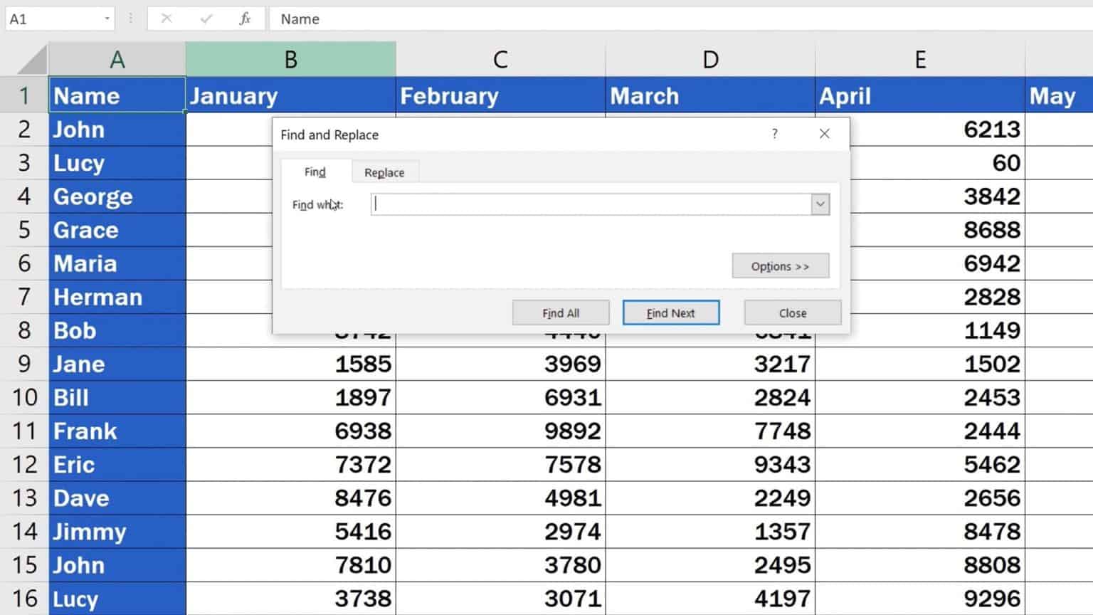
• Press Ctrl + F on Windows or Command + F on Mac to launch the Find and Replace dialog box. Alternatively, go to the Home tab and click Find & Select > Find.

• In the Find what field, type the text or value you want to search for.

• Click Find Next to jump to the first occurrence or Find All to see a list of all occurrences.

• When you locate what you want, click Replace to swap it out with new text.

The Find tool works great for quick searches. But you can refine the search further using wildcard characters…

Leverage Wildcard Characters

Wildcard characters act like placeholders to find values that match a certain pattern. Here are the most useful ones:

• Asterisk (*) – Finds any text that matches the characters before and after it. For example, s*t finds sit, sat, start etc.

• Question mark (?) – Matches any single character in that position. b?g finds bag, big, bug etc.

• Tilde (~) – Cancels any special meaning of the character after it. To find a literal *, use ~*.

Using wildcards makes searching more flexible. You can find words, numbers and patterns even when you don’t know the exact text.

Search Within Specific Criteria

The Find tool also lets you filter the search by certain criteria:

• Search within a specific sheet or the entire workbook

• Look in values, formulas, or comments

• Match entire cell contents or partial cell contents

• Match case or ignore case

• Search by row or column

To access these options, open the Find tool and click Options. Then check the boxes for your preferred criteria before starting the search.

This filtering prevents false matches and narrows the results to only what you need.

Use AutoFilter to Search Data

Excel’s AutoFilter tool is perfect for searching and analyzing tabular data. Here are the steps:

• Select the data you want to filter

• Go to Data > Filter

• Arrows appear in the header of each column

• Click the arrow in the column you want to search and check the boxes next to values you want to filter by

• The table will instantly filter, showing only rows with the selected values

• Once filtered, you can sort by column, copy visible cells, and more

AutoFilter is extremely fast for searching datasets. You can also filter by colors, cell icons, duplicate values and other criteria.

Create Custom Filters with Advanced Options

For more complex filtering, use the Advanced filter option:

• Select your data range

• Go to Data > Sort & Filter > Advanced

• In the Advanced Filter window, define your search criteria

• Options include filtering by values, dates, duplicates, formulas, cell colors and icons

• You can copy filtered results to another location or overwrite visible cells

With Advanced filtering, you can create AND/OR logic and show records that match two or more criteria. This gives you pinpoint control.

Lookup Data with VLOOKUP

VLOOKUP is an Excel function great for crosstab-style lookups. Here’s the syntax:

=VLOOKUP(Search Key, Range, Column Number, Exact Match)

• Search Key is the value you want to find

• Range is the table or range to search

• Column Number is the column with data to return

• Exact Match is TRUE for exact matches only or FALSE for approximate

For example:

=VLOOKUP(A2,D:E,2,FALSE) looks in columns D and E to find the value in A2. It returns the corresponding value from column E.

VLOOKUP pulls data from one place to another. Similar to a database search.

Search Horizontally with HLOOKUP

HLOOKUP works the same as VLOOKUP but searches horizontally instead of vertically:

=HLOOKUP(Search Key, Range, Row Number, Exact Match)

• Search Key, Range and Exact Match work the same

• Row Number is the row in the range containing the return value

For example:

=HLOOKUP(B1,B1:E10,3,FALSE) looks across row 3 to find B1. It returns the value from column C.

HLOOKUP is useful when your data is arranged horizontally instead of vertically.

Use INDEX/MATCH for Flexible Lookups

INDEX/MATCH gives you more flexibility than VLOOKUP alone. The INDEX function returns a value from a range but lets you specify the return value’s exact position.

We pair this with MATCH to find the position:

=INDEX(Return Range, MATCH(Search Key, Search Range, 0))

• Return Range is the table/range containing the data to return

• Search Range is the place to search for the key

• Search Key is the lookup value

• MATCH finds the position of key in the search range

Some advantages over VLOOKUP:

• Lookup columns to the left
• Return from any row or column
• Handle duplicate keys
• Perform partial match lookups

Master INDEX/MATCH and unlock powerful lookup abilities!

Use Navigation Shortcuts

Don’t forget Excel’s handy keyboard shortcuts for fast navigation:

• Ctrl + Arrow Keys – Move between cells
• Ctrl + Shift + Arrow Keys – Select cells
• Ctrl + Home – Go to beginning of sheet
• Ctrl + End – Go to bottom of sheet
• Page Up/Down – Move one screen up/down

Combine these with searching to zip around large sheets and inspect matching cells.

Master Useful Shortcuts

Along with navigation shortcuts, memorize these for efficient searching:

• F5 – Open Go To dialog to select a specific cell
• Ctrl + G – Also opens the Go To dialog
• Ctrl + P – Launch print preview to visually scan sheet
• Alt + H + L – Select visible cells after filtering
• Ctrl + A – Select all cells to inspect the full sheet

Work these into your flow to save time.

Final Tips and Tricks

Here are a few more tips for mastering search in Excel:

• Search column by column to catch vertical duplicates
• Add column headers for crucial context
• Color code key data types like dates, names, addresses
• Split data into multiple sheets for easier scanning
• Freeze top rows so headers remain visible when scrolling
• Customize conditional formatting rules to highlight findings

Get creative with formats, shortcuts and formulas to optimize your workflow.

With this full guide under your belt, you can find any information you need – even in giant Excel data sets. Just remember the search basics:

• Use Find, wildcards and filters to zero in on text and values

• Fetch data from one place to another with lookup functions

• Build custom logic with helper columns

• Speed up navigation with keyboard shortcuts

• Color code and structure your sheets strategically

Soon you’ll be searching spreadsheets quicker than Ctrl+F! But if you ever get stuck, refer back to this manual.