The tutorial will teach you two quick ways to randomize in Excel: perform random sort with formulas and shuffle data by using a special tool.
Microsoft Excel provides a handful of different sorting options including ascending or descending order, by color or icon, as well as custom sort. However, it lacks one important feature – random sort. This functionality would come in handy in situations when you need to randomize data, say, for an unbiased assigning of tasks, allocation of shifts, or picking a lottery winner. This tutorial will teach you a couple of easy ways to do random sort in Excel.
Do you have a list in Excel that you want to randomize? Randomizing a list in Excel is easy with just a few simple steps
Whether you want to shuffle names, numbers, or labels, this comprehensive guide will show you how to randomize rows in Excel using formulas for truly random sorts.
Why Randomize a List in Excel?
Here are some common reasons you may want to randomize a list in Excel:
-
Randomly assigning test variants in A/B testing experiments.
-
Shuffling a list of names when picking sweepstake winners.
-
Mixing up a list of tasks or to-do items to prevent bias.
-
Randomizing quiz questions so each student gets a different order.
-
Creating a randomized playlist for music/videos.
-
Random sampling for statistical analysis.
-
Shuffling teams or players in games and sports.
Randomizing removes any inherent order and ensures everyone has an equal chance. Now let’s see how to easily achieve this in Excel.
How to Quickly Randomize a List in Excel
While Excel doesn’t have a built-in “randomize list” feature you can add randomness in 3 simple steps
Step 1: Insert a Column with the RAND Formula
-
Insert a new blank column next to your list
-
In the new column, enter the
=RAND()formula in the first cell -
Drag the formula down to return random numbers next to each row
Step 2: Sort the Formula Column
-
Select the column with RAND formulas
-
Go to Data > Sort to sort the random numbers
-
Choose ascending or descending order
Step 3: Delete the Formula Column
-
Once your list is randomized, delete the column with RAND formulas
-
You’re left with a randomly sorted list without random numbers!
This easy trick works for randomizing any data set in Excel. The RAND formula generates the randomness while sorting propagates that to shuffle your list.
Breaking Down the RAND Formula
The RAND() formula is vital for randomizing lists in Excel. Here’s what you need to know:
-
RAND()generates a random decimal number between 0 and 1. -
It recalculates whenever the worksheet is calculated.
-
The output changes randomly on each cell recalculation.
-
Being a volatile function,
RAND()keeps providing random numbers. -
No inputs or arguments are needed – just enter
RAND()! -
Available in all versions of Excel.
The RAND formula brings true randomness into your data. Combined with sorting, it lets you easily shuffle any list.
Step-By-Step Guide to Randomize Lists in Excel
Let’s walk through a detailed example of randomizing a list in Excel:
-
Start with a list of data to randomize. This could be names, email IDs, quiz questions etc.
-
Insert a new blank column next to it. This will contain the RAND formulas.
-
In the first cell of the new column, enter
=RAND(). Copy this down the entire column. -
You’ll now have a column of random decimal numbers next to your list.
-
Select this column and go to Data > Sort.
-
Choose to sort Smallest to Largest or Largest to Smallest. Click OK.
-
The list will now be randomized based on the random sort order.
-
Delete the column containing RAND formulas.
-
Done! Your list is now randomly shuffled.
This process works for randomizing any data set in Excel with just a few clicks.
Randomizing Lists Using RANDBETWEEN
Apart from RAND, you can also use the RANDBETWEEN function to randomize lists in Excel.
RANDBETWEEN returns a random whole number between specified limits. For randomizing lists, you can use:
=RANDBETWEEN(1,100)This generates random integers from 1 to 100.
The steps are same as RAND – insert a column with RANDBETWEEN formulas, sort it, and then delete it once your list randomizes.
Randomly Sampling Data in Excel
For statistical sampling, you can use the above approach to select random rows from Excel datasets:
-
Let’s say you want a random sample of 10 rows from 100 rows of data.
-
Insert a column with
=RAND()formulas to assign random numbers. -
Sort this column to shuffle the dataset randomly.
-
Select and copy the first 10 rows as your random sample.
Random sampling gives you an unbiased, representative subset for analysis.
Adding Randomness When Selecting Multiple Items
To select multiple random items from a list (say 5 winners from 100):
-
Add RAND column and sort randomly
-
Enter
=RAND()in an empty cell -
Use top 5 values in the formula column to match rows in randomized list
-
Top 5 rows with same random values are the random winners!
The additional RAND column provides the linkage between random numbers and list items.
Randomizing List Without Formulas
Here are some alternatives to generate randomness without adding formula columns:
-
Apply conditional formatting using =RAND() rule. Sort by cell color.
-
Add Data > Filter to create random sort orders.
-
Use dynamic arrays – FILTER to extract randomized rows.
-
Copy the list to another location, shuffle rows manually.
However, the RAND formula method is easiest and most foolproof for true randomness.
Chart Showing Randomized List in Excel
Here is a chart depicting the entire process flow to randomize lists in Excel using the RAND formula:
![Randomize list chart]
Things to Remember
While randomizing lists is straightforward in Excel, keep these tips in mind:
-
Formulas recalculate so don’t overwrite randomized data.
-
Manually sorting again will mess up randomization.
-
Use new random numbers if you want to reshuffle.
-
Test for sufficient randomness using statistical tests.
-
Avoid rand() on entire columns which slows down Excel.
-
Make sure you delete random number columns once done.
Advanced: VBA Code to Randomize Lists
You can also write a VBA macro to randomize lists automatically in Excel.
For example:
Sub RandomizeList() Dim rng As Range Set rng = Range("A2:A100") 'List to Randomize 'Shuffle Code For i = 1 To 100 rng.Cells(i).Value = rng.Cells(Rnd() * 100 + 1) Next i End SubThis macro loops through the list range, assigns a random cell value to each row, and loops again. This continues for 100 iterations to shuffle your list randomly.
You can customize the row count and target range as needed.
So in a few lines of VBA code, you can easily mimic the manual steps for randomizing lists in Excel.
Applications of Randomized Lists
Here are some examples of how you can use randomized lists in Excel for different tasks:
-
Randomly assign test groups for A/B testing.
-
Shuffle names when picking sweepstakes or contest winners.
-
Mix up playlists for music, podcasts, or YouTube.
-
Randomly sample data for surveys, statistics etc.
-
Create randomized quizzes by shuffling question order.
-
Randomly generate training/test datasets for machine learning.
-
Mix up sports/game opponents, players, or maps.
No matter what you want to randomize, Excel provides the tools to easily shuffle any list or sequence.
Tips for Random Sorting
Here are some tips for effective randomization of lists in Excel:
-
Use a column of RAND or RANDBETWEEN formulas to generate numbers.
-
Sort the column to shuffle your list randomly.
-
Check formulas recalculate properly after sorting.
-
Delete random number columns once list is shuffled.
-
Test randomness by sorting a few times.
-
Don’t overwrite your randomized data.
-
Avoid full column formulas as it slows Excel.
-
Use new random numbers if reshuffling the same list.
Key Takeaways
The key points about randomizing lists in Excel are:
-
Add a column with RAND() or RANDBETWEEN() formulas
-
Sort this column to shuffle your list into a random order
-
Remove the column with random formulas once done
-
The RAND() formula brings true randomness for random sorting
-
Alternatives include conditional formatting, filtering etc.
-
Useful for A/B tests, surveys, games, statistics etc.
So with just basic Excel skills and RAND formulas, you can easily randomize any dataset.
With this simple yet powerful technique, shuffling lists for unbiased analyses becomes a breeze in Excel!
How to randomize a list in Excel with a formula
Although there is no native function to perform random sort in Excel, there is a function to generate random numbers (Excel RAND function) and we are going to use it.
Assuming you have a list of names in column A, please follow these steps to randomize your list:
- Insert a new column next to the list of names you want to randomize. If your dataset consists of a single column, skip this step.
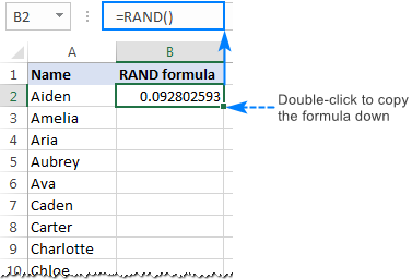
- In the first cell of the inserted column, enter the RAND formula: =RAND()
- Copy the formula down the column. The fastest way to do this is by double-clicking the fill handle:
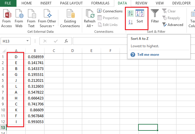
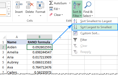
- Sort the column filled with random numbers in ascending order (descending sort would move the column headers at the bottom of the table, you definitely dont want this). So, select any number in column B, go to the Home tab > Editing group and click Sort & Filter > Sort Largest to Smallest.
 Or, you can go to the Data tab > Sort & Filter group, and click the ZA button
  .
.
Either way, Excel automatically expands the selection and sorts the names in column A as well: 
Tips & notes:
- Excel RAND is a volatile function, meaning that new random numbers are generated every time the worksheet is recalculated. So, if you are not happy with how your list has been randomized, keep hitting the sort button until you get the desired result.
- To prevent the random numbers from recalculating with every change you make to the worksheet, copy the random numbers, and then paste them as values by using the Paste Special feature. Or, simply delete the column with the RAND formula if you dont need it any longer.
- The same approach can be used to randomize multiple columns. To have it done, place two or more columns side by side so that the columns are contiguous, and then perform the above steps.
How to shuffle data in Excel with Ultimate Suite
If you dont have time to fiddle with formulas, use the Random Generator for Excel tool included with our Ultimate Suite to do a random sort faster.
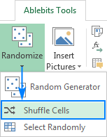
- Head over to the Ablebits Tools tab > Utilities group, click the Randomize button, and then click Shuffle Cells.
- The Shuffle pane will appear on the left side of your workbook. You select the range where you want to shuffle data, and then choose one of the following options:
- Cells in each row – shuffle cells in each row individually.
- Cells in each column – randomly sort cells in each column.
- Entire rows – shuffle rows in the selected range.
- Entire columns – randomize the order of columns in the range.
- All cells in the range – randomize all cells in the selected range.
- Click the Shuffle button.
In this example, we need to shuffle cells in column A, so we go with the third option: 
And voilà , our list of names is randomized in no time: 
If you are curious to try this tool in your Excel, you are welcome to download an evaluation version below. Thank you for reading!
How to Randomize a List In Excel
How to randomize a list in Excel?
For example, we want to randomize the list in column A below. 1. Select cell B1 and insert the RAND () function. 2. Click on the lower right corner of cell B1 and drag it down to cell B8. 3. Click any number in the list in column B. 4. To sort in descending order, on the Data tab, in the Sort & Filter group, click ZA. Result.
How to sort based on random numbers in Excel?
Choose either the Sort Ascending or Sort Descending option. Now that the data is sorted based on the random column, it’s no longer needed and you can delete it. Right-click on the Order column heading containing the random numbers. Select the Remove option from the menu. Now the query can be loaded into Excel.
How to shuffle a list of random names in Excel?
In case you want to shuffle this list again, hit the F9 key and the list would shuffle again (this happens because RANDARRAY is a volatile function and refreshes whenever you hit F9 or make a change in the Excel file) Once you have the list of random names you want, you can convert the formula to values so that it doesn’t change again.
