After youve entered data into Google Sheets, you may want to create a visualization of that information to make it easier to convey. Luckily, Google Sheets makes it easy for you to convert data into a graph or chart. Easy as Raspberry Pi, if you will.
Google Sheets gives you a variety of options for your graph, so if you want to show parts that make up a whole you can go for a pie chart, and if you want to compare statistics, a bar graph will likely make more sense. Here are our step-by-step instructions for making a graph in Google Sheets.
1. Select cells. If youre going to make a bar graph like we are here, include a column of names and values and a title to the values.
4. Select which kind of chart. Pie charts are best for when all of the data adds up to 100 percent, whereas histograms work best for data compared over time.
5. Click Chart Types for options including switching what appears in the rows and columns or other kinds of graphs.
With Google Sheets, you can easily create different types of charts and graphs to visualize your data Charts allow you to present spreadsheet data in a graphical format for better analysis and insights
In this comprehensive guide, I’ll walk through the steps options, and tips for making charts in Google Sheets using both desktop and mobile apps.
Why Make Charts in Sheets
Here are some of the top reasons to use charts in Google Sheets:
- Visualize data trends, patterns and insights.
- Simplify data analysis compared to studying sheets.
- Identify data outliers and exceptions easily.
- Present summarized data concisely to others.
- Embed charts to provide context in reports and dashboards.
- Mix and match different chart types for multi-dimensional data.
Adding charts takes your sheet data from plain numbers and labels to interactive visual depictions that give you a whole new perspective.
How to Create a Chart in Sheets
Follow these steps to turn sheet data into a chart in Google Sheets:
-
Select data – Highlight the cells containing the data you want to chart.
-
Click Insert > Chart – Pick from column, bar, line, pie and more.
-
Customize layout – Edit the chart title, legend, axis labels and more.
-
Refine chart – Adjust scale, data labels, colors, fonts to perfect the chart.
-
Position chart – Place the chart on the sheet or its own page.
That’s all there is to it! Now let’s look at the steps and options in more detail.
Chart Data Selection Tips
-
Only select column or row data, not individual cells.
-
Headers can be included to label charts.
-
Multiple series can be charted from adjacent columns.
-
Allow for captions by adding a blank row above.
-
Too much data will clutter charts. Filter down if needed.
Carefully selecting your source data is key to great looking charts.
Picking Your Google Sheets Chart Type
Google Sheets supports these chart types to match your data:
-
Column – Vertical bars for comparing categories.
-
Bar – Horizontal bars better for longer text labels.
-
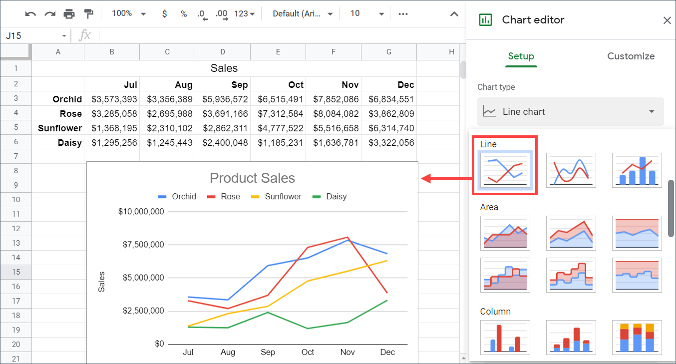
Line – Connected data points showing trends and progressions.
-
Pie – Circular divided segments displaying value proportions.
-
Scatter – Plotted coordinate data pairs and correlations.
-
Histogram – Frequency distribution of numeric data buckets.
-
Combo – Hybrid charts with mixed types.
Pick the type that best represents your data and goals. The default will often work great.
Customizing and Editing Your Chart
Take full control over chart layout and design:
-
Add chart and axis titles – Describe what’s shown.
-
Modify legend – Change position, labels, icons.
-
Edit labels – Rotate, reformat, or add custom labels.
-
Adjust scale and axis – Set min/max values, units and increments.
-
Switch aggregation – Change how data is rolled up.
Don’t settle for default charts. Tailor them to perfectly fit your data!
Formatting Chart Elements
Refine chart appearance by formatting elements:
-
Set fill colors – Use color scales, gradients, and patterns.
-
Modify font styles – Make titles stand out from labels.
-
Add borders – Clearly separate bars or slices.
-
Show data labels – Annotate chart data points directly.
-
Set transparency – Mute chart colors for distinction from grid.
Subtle formatting tweaks can take your charts to the next level visually.
Smoothing Chart Data
Make charts easier to read by smoothing the data:
-
Use rolling averages – Soften volatile trends and fluctations.
-
Employ trendlines – Show overall trajectory ignoring dips.
-
Apply outlier cleanup – Remove anomalies throwing off axis.
-
Set log scale – Compress extreme value variance.
Smoothed charts emphasize long term patterns over temporary blips.
Positioning Charts on Sheets
Place your charts for maximum impact:
-
On same sheet – Embed amongst grid data for direct context.
-
New sheet – Plot on dedicated chart page for singular focus.
-
Dashboard – Combine with other charts for overview.
-
Linked copies – Duplicate charts showing dynamic data updates.
Think about chart placement in terms of how they’ll be viewed.
Creating Charts in Sheets Mobile Apps
The Google Sheets mobile apps make charting on the go easy:
-
Tap cells – On Android or iOS, select data then tap Insert > Chart.
-
Pick chart – Switch between column, bar, line, pie and more.
-
Edit and format – Customize titles, labels, colors and size.
-
Touch actions – Drag slices, scroll axis, zoom charts interactively.
The mobile apps provide a streamlined charting experience optimized for smaller touchscreens.
Copying Charts to Other Files
Rather than recreating the same chart repeatedly:
- Save as template – Define a reusable blank chart
How To Make A Chart In Google Sheets
How do I create a chart in Google Sheets?
Another option is to insert a chart from Google Sheets, a new feature from summer 2016. First, make the chart from your data in your Google Sheets spreadsheet. Then, in Google Docs, select Insert -> Chart -> From Sheets… to add that chart to your Google Docs document.
How to make a pie chart in Google Sheets?
On your computer, open a spreadsheet in Google Sheets. Double-click the chart you want to change. At the right, click Customize. Choose an option: Chart style: Change how the chart looks. Pie chart: Add a slice label, doughnut hole, or change border color. The following six steps will show you how to make a pie chart in Google Sheets: 1.
How do I add a title to a chart?
To add a title, simply click on the chart and select “Chart Title” from the “Chart Layout” tab. You can then enter your desired title and adjust the font, size, and color as needed. To add labels to your chart, select one of the sections and right-click on it.
