Charts are a great way to share data and information in a graphical way. The foundation of charts is the data they illustrate. Choosing the right data is the first and most important step in creating a chart.
Once youve determined the results you want your chart to display, choose the chart that best suits this purpose. The most popular charts are column, line, pie, and bar charts.
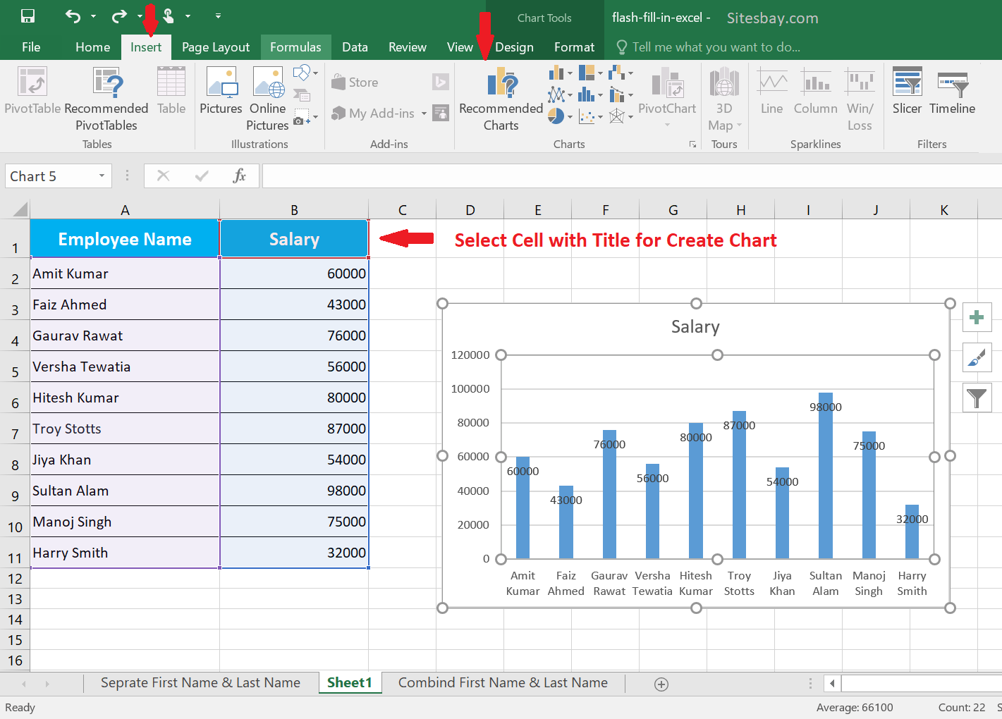
The chart appears in the worksheet and the Chart Tools appear on the Ribbon. The Chart Tools include three new tabs—Design, Layout and Format—that help you modify and format the chart.
Many times, it’s hard to tell what type of chart will best illustrate your data. To help make your decision easier, Excel offers Recommended Charts. This tool looks at the data you have selected and suggests a few charts that will represent it well.
Charts and graphs are a great way to visualize data and convey information quickly. With just a few clicks, you can create a variety of charts and graphs in Excel to turn raw data into meaningful insights.
In this comprehensive guide I’ll walk you through the entire process of creating professional-looking charts in Excel from selecting your data to customizing the final chart. Whether you’re a complete beginner or an experienced Excel user, you’ll learn some useful tips and tricks for making eye-catching, informative charts.
Step 1: Select the Data for Your Chart
The first step is to select the data you want to use for the chart. This includes both the x-axis categories (for column, bar, and line charts) and the data series.
Here are a few things to keep in mind when selecting data:
-
Data should be organized with labels in the first row and column. This makes it easier for Excel to recognize the data ranges.
-
Avoid including blank rows or columns in your selection. This can distort the chart.
-
You can select data from multiple rows or columns, but they need to align properly. For example, if your first data series is in columns A and B, the second one must be in C and D.
-
Ctrl + click to select non-adjacent columns. Or, click and drag to select a range of adjacent cells.
Once your data is selected, you’re ready to create the chart!
Step 2: Insert a Chart
With your data selected, go to the Insert tab on the Excel ribbon and click the Recommended Charts button. This will open a window showing chart suggestions based on your data:
![Recommended Charts window][]
- On the left, you’ll see chart types that Excel recommends. Click each one to see a preview on the right.
- Once you find the chart you want, click it and select OK.
Alternatively, you can click a specific chart type on the Insert tab. Column, bar, line, pie, scatter, and more – the options are all there!
After selecting a chart type, it will appear on your worksheet, ready to be customized.
Step 3: Switch Rows and Columns (If Needed)
One common formatting change is to switch the rows and columns.
For example, if your data has categories in rows and data series in columns, your chart’s x-axis will show the categories. By switching the rows and columns, you can make the data series appear on the x-axis instead.
To switch rows and columns:
- Select the chart.
- Go to the Design tab.
- Click Switch Row/Column button.
This will instantly pivot the axes, putting the data series horizontally and categories vertically.
Step 4: Change the Chart Type
Don’t like the chart type you picked? No worries – it’s easy to change to a different one.
With your chart selected:
- Go to the Design tab.
- Click Change Chart Type.
- Select the desired chart from the left pane.
- Click OK.
The chart will change to the new type while preserving colors, labels, and other customizations. Feel free to experiment until you find the ideal chart for your data!
Step 5: Add Chart Elements
Most charts look pretty plain at first. Here are some common elements you can add:
- Chart title – Summarizes the purpose of the chart. Click above the chart and type a descriptive title.
- Axes titles – Label the units and categories on each axis. Double-click an axis title to edit it.
- Legend – Identifies data series in the chart. To add, click the + on the chart and check Legend.
- Data labels – Show values next to data points. Select a data series, click +, and check Data Labels.
- Gridlines – Add horizontal and vertical lines for scale. Click + and check Gridlines.
- Trendline – Shows the linear trend of data. Right-click a data series and select Add Trendline.
Add and arrange elements by clicking the + button on the chart and checking the boxes.
Step 6: Customize the Look and Style
Once your chart is fully labelled, it’s time for the fun part – making it look snazzy! Here are some customizations to try:
- Change colors – For the whole chart or individual data series. Go to Format > Fill & Line options.
- Add chart styles – Try different backgrounds, colors, and effects. Go to Design > Chart Styles.
- Format text – Customize fonts, size, color, etc for titles and labels. Go to Format > Text options.
- Resize and position – Click and drag the edge or corners to resize. Drag the chart to move it.
- Add images – Right-click the chart, select Edit Data, and insert a picture in Image files.
- Annotate – Draw attention to insights by adding text boxes, arrows, and shapes.
Don’t be afraid to try bold colors, effects, and layouts. Just remember to maintain clear labeling and legibility.
Advanced Chart Features
Once you’ve mastered the basics, try some of these advanced features:
- Combo chart – Combine different chart types like a column and line chart.
- Secondary axis – Add a secondary vertical axis for two different data scales.
- Error bars – Show variability for each data point. Right-click > Format Data Series > Y Error Bars.
- Trendlines – Add linear or exponential trendlines to data series. Right-click > Add Trendline.
- Moving average – Smooth out fluctuations in time-series data. Click data series > Add > Moving average.
- Sparklines – Add mini charts alongside cells of data. Go to Insert > Sparklines.
- Waterfall chart – See how positive and negative values add up. Click Insert > Recommended Charts > Waterfall.
- Histogram – Count occurrences within data ranges. Click Insert > Histogram.
Don’t limit yourself – explore all the options under the Chart Tools and Design tabs. Knowing how to make charts in Excel gives you the power to turn any dataset into a powerful visualization.
Tips for Creating Effective Excel Charts
Follow these best practices and your Excel charts will look clean, professional, and convey information clearly:
- Label everything – Axis titles, data labels, legend. Leave no question what the data means.
- Link to source data – If data changes, the chart updates automatically if linked.
- Avoid clutter – Only keep essential text, elements, and data. Remove gridlines, borders, and unnecessary legend entries.
- Use appropriate chart type – Bar for comparison, line for trends, pie for proportions, scatter for correlations, etc.
- Make judicious use of color – Use sparingly and with purpose. Make sure colors contrast.
- Watch font sizes – Text should be readable. Format axis labels and legend differently than titles.
- Include context – Add context in titles,
Excel Charts and Graphs Tutorial
How do I create a chart?
Charts help you visualize your data in a way that creates maximum impact on your audience. Learn to create a chart and add a trendline. You can start your document from a recommended chart or choose one from our collection of pre-built chart templates. Select data for the chart. Select Insert > Recommended Charts.
How do I make a graph in Excel?
This wikiHow tutorial will walk you through making a graph in Excel. Open a Blank workbook in Excel. Click Insert chart. Select the type of graph you want to make (e.g., pie, bar, or line graph). Plug in the graph’s headers, labels, and all of your data. Click and drag your mouse to select all your data, then click Insert.
How to create a line chart in Excel?
To create a line chart, execute the following steps. 1. Select the range A1:D7. 2. On the Insert tab, in the Charts group, click the Line symbol. 3. Click Line with Markers. Result: Note: enter a title by clicking on Chart Title. For example, Wildlife Population. You can easily change to a different type of chart at any time. 1. Select the chart.
How do I create a recommended chart in Excel?
Select data for the chart. Select Insert > Recommended Charts. Select a chart on the Recommended Charts tab, to preview the chart. Note: You can select the data you want in the chart and press ALT + F1 to create a chart immediately, but it might not be the best chart for the data.
