In this tutorial, you will learn how to make a bar graph in Excel and have values sorted automatically descending or ascending, how to create a bar chart in Excel with negative values, how to change the bar width and colors, and much more.
Along with pie charts, bar graphs are one of the most commonly used chart types. They are simple to make and easy to understand. What kind of data are bar charts best suited for? Just any numeric data that you want to compare such as numbers, percentages, temperatures, frequencies or other measurements. Generally, you would create a bar graph to compare individual values across different data categories. A specific bar graph type called Gantt chart is often used in project management programs.
In this bar chart tutorial, we are going to explorer the following aspects of bar graphs in Excel:
Making bar graphs in Excel is a great way to visualize data and make it more engaging than just looking at a spreadsheet. Bar graphs are easy to read and understand, allowing you to quickly compare values. In this comprehensive guide, I’ll walk you through the entire process of making a bar graph in Excel from entering your data to customizing the final look.
Why Use a Bar Graph in Excel?
Before jumping into the steps let’s first go over some of the key reasons you’d want to make a bar graph in Excel
-
Visually compare values or categories: Bar graphs allow you to see at a glance how values or categories compare to each other. This makes it easy to spot trends and relationships.
-
Engage your audience Bar graphs are more dynamic and interesting to look at than raw data. Using bar graphs helps keep your audience engaged
-
Save time: Once your data is entered, it only takes a few clicks to create a bar graph in Excel. It’s a fast and simple way to visualize your data.
-
Easy to understand: Bar graphs are intuitive charts that most people can interpret easily. They clearly show magnitude and comparisons.
-
Flexible: You can customize Excel bar graphs in many ways to best display your data. For example, you can change the color scheme and layout.
Step 1: Enter Your Data in Excel
The first step is to enter your raw data into Excel cells. You can insert a bar graph using any existing Excel data, but your data must be structured properly:
-
Put category labels in the first column (e.g. days of the week).
-
Put values you want to compare in the second column (e.g daily temperatures).
-
Each row should contain a paired category and value.
It’s common to add axis labels in the top row, like “Day” and “Temperature”. This clearly defines what’s being compared.
Here’s an example structured data table in Excel to use for a bar graph:
| Day | Temperature |
|---|---|
| Monday | 65 |
| Tuesday | 71 |
| Wednesday | 80 |
| Thursday | 75 |
| Friday | 68 |
This table compares temperatures over the days of the week. Now we can make a bar graph to visualize it.
Step 2: Select Your Data
Next, select the data you want to use for the bar graph. An easy way is:
-
Click the top-left cell of your data table.
-
Scroll down and Shift + Click the bottom-right cell to select the full range.
Alternatively, you can manually drag your mouse over all the cells. Just be sure your category labels and data values are all included in the selection.
Step 3: Insert a Bar Chart
With your data selected, go to the Insert tab and click the Bar Chart icon:
![Bar chart icon in Excel][]
This opens various bar chart options to insert. For a basic bar graph, choose a 2-D Column chart:![2D Column chart][]
And there we have it! A bar graph is inserted from the selected data. By default, Excel does a great job constructing the chart.
Step 4: Customize and Format the Bar Graph
If needed, you can customize the look and layout of your Excel bar graph to perfection. Here are some common formatting options:
- Swap axes: The “Switch Row/Column” button swaps the axes, changing to a horizontal bar graph.
- Change bar colors: Update colors under the “Colors” section.
- Add chart titles/labels: Edit the default text by clicking it.
- Modify scale: Adjust how the value axis is displayed under “Axis options”.
- Change font styles: Update text fonts and colors using the formatting toolbar.
- Add visual effects: Make bars 3D, add borders, fill areas, and more under “Shape Styles”.
Take time to play around with the different formatting options in the toolbar to get your graph looking just right.
Tips for an Effective Bar Graph
To create more effective and visually appealing Excel bar graphs, keep these tips in mind:
- Display no more than 8-10 bars. Too many makes it cluttered.
- Order bars logically, like largest to smallest or chronologically.
- Make the most important bar darker to draw attention.
- Include concise but descriptive axis titles and graph title.
- Add data labels directly on the bars to show exact values.
- Show trends by using consistent bar colors across groups.
- Keep it simple. Only use 3D, shadows, etc. if they add value.
Common Bar Graph Types
Beyond the basic column bar chart, there are a few other common types of bar graphs you can insert in Excel:
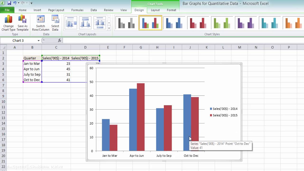
- Grouped Bar Graph: Compares values across multiple groups or categories using clustered bars. Useful for time series data.
- Stacked Bar Graph: Displays parts of a whole stacked on each bar, like components of a total. Helps visualize part-to-whole relationships.
- 100% Stacked Bar Graph: Same as stacked, but each bar totals 100% to show percentages or proportions.
- Horizontal Bar Graph: Flips the orientation, with bars going horizontal rather than vertical. Helps if you have long category names.
The steps to create any of these alternative bar graph formats are the same. Just select the desired chart type when inserting your bar chart.
Bar Graphs vs Other Chart Types
Bar graphs are great for many situations, but aren’t always the best way to present data visually. Here are a few other Excel chart types to consider:
- Column charts: Essentially the same as bar graphs but with vertical columns instead of horizontal bars. Use for smaller datasets.
- Line charts: Useful for visualizing trends over time. Lines can plot continuous data.
- Pie charts: Display parts of a whole. Better for seeing percentages or proportions.
- Scatter plots: Plot relationships between two numeric variables. Useful for correlation data.
The key is to select the chart format that will best help viewers understand your data. Try different types to see which works best. Bar graphs are a good starting point for categorical data.
Advanced Tips and Tricks
Here are a few more advanced bar graph techniques for Excel power users:
- Use VBA macros to automate generating bar graphs from datasets.
- Link bar graphs to cells so they update when you change the source data.
- Create combo charts with bars and lines to compare two data series.
- Add error bars, trendlines, regression, and other statistical analysis.
- Make dynamic, interactive bar graphs with form controls, like scrollbars linked to cell values.
- Use PivotTables and PivotCharts to easily sort, filter, and update bar graphs.
The more you work with bar graphs in Excel, the more ways you’ll find to customize, optimize, and enhance them for your needs.
Troubleshooting Common Bar Graph Issues
At times, your Excel bar graphs may not turn out quite right. Here are solutions for some common problems:
- Bars in wrong order: Ensure your data is sorted properly in the source table.
- Too many bars: Reduce clutter by hiding extra columns before inserting the graph.
- Gaps between bars: Increase the overlap under “Series Options”.
- Bars not aligned: Fix by setting axis bounds under “Axis Options”.
- Bar width not right: Increase/decrease the gap width until bars are desired width.
- Colors changed: Reapply your desired color scheme.
- Axis scales off: Change minimum and maximum values under axis settings.
- Bars overlapping: Reduce overlap for clearer separation.
With a bit of tweaking, you can resolve most bar graph issues that come up.
Key Takeaways
To recap, here are some key points for creating great-looking bar graphs in Excel:
- Structure your source data properly with categories and values.
- Select the full data range, then insert a 2-D bar chart.
- Customize the color, layout, font, scale, and other formatting.
- Order bars logically, limit to 8-10, make one stand out.
- Consider other chart types like lines or columns if needed.
- Take advantage of advanced features for power users.
- Quickly troubleshoot issues like order, gaps, alignment, and overlap.
Making compelling, informative bar graphs in Excel is easy with a few simple steps. Hopefully this guide has equipped you with all the
Create Excel bar charts with negative values
When you make a bar graph in Excel, the source values do not necessarily need to be greater than zero. Generally, Excel has no difficulty with displaying negative numbers on a standard bar graph, however the default chart inserted in your worksheet might leave much to be desired in terms of layout and formatting: 
For the above bar chart to look better, firstly, you might want to move the vertical axis labels to the left so they wont overlay the negative bars, and secondly, you can consider using different colors for negative values.
To format the vertical axis, right click any of its labels, and select Format Axis… from the context menu (or simply double-click the axis labels). This will make the Format Axis pane appear on the right side of your worksheet.
On the pane, go to the Axis Options tab (the rightmost one), expand the Labels node, and set the Label Position to Low: 
If you want to draw attention to the negative values in your Excel bar graph, changing the fill color of negative bars would make them stand out.
If your Excel bar chart has just one data series, you can shade negative values in standard red. If your bar graph contains several data series, then you will have to shade negative values in each series with a different color. For example, you can keep the original colors for positive values, and use lighter shades of the same colors for negative values.
To change the color of negative bars, perform the following steps:
- Right click on any bar in the data series whose color you want to change (the orange bars in this example) and select Format Data Series… from the context menu.
- On the Format Data Series pane, on the Fill & Line tab, check the Invert if Negative box.
- As soon as you put a tick in the Invert if Negative box, you should see two fill color options, the first for positive values and the second for negative values.
Tip. If the second fill box does not show up, click the little black arrow in the only color option that you see, and choose any color you want for positive values (you can select the same color as was applied by default). Once you do this, the second color option for negative values will appear: 
Change the bar width and spacing between the bars
When you do a bar graph in Excel, the default settings are such that theres quite lot of space between the bars. To make the bars wider and get them to appear closer to each other, perform the following steps. The same method can be used to make the bars thinner and increase the spacing between them. In 2-D bar charts, the bars can even overlap each other.
- In your Excel bar chart, right click any data series (the bars) and choose Format Data Series… from the context menu.
- On the Format Data Series pane, under Series Options, do one of the following.
- In 2-D and 3-D bar graphs, to change the bar width and spacing between data categories, drag the Gap Width slider or enter a percentage between 0 and 500 in the box. The lower the value, the smaller the gap between the bars and thicker the bars, and vice versa.
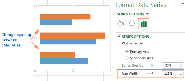
- In 2-D bar charts, to change the spacing between data series within a data category, drag the Series Overlap slider, or enter a percentage between -100 and 100 in the box. The higher the value, the greater the bars overlap. A negative number will result in a spacing between the data series like in the following screenshot:

- In 3-D charts, to change the spacing between data series, drag the Gap Depth slider, or enter a percentage between 0 and 500 in the box. The higher the value, the greater the gap between the bars. In practice, changing the gap depth does have a visual effect in most of Excel bar chart types, but it does make a noticeable change in a 3-D column chart, as shown in the following :

How to Make a Bar Graph in Excel
How to make a bar graph in Excel?
To make a bar graph in Excel: Select the data to be plotted in the bar graph. Go to the Insert tab in the ribbon > Charts group. You will see different chart types in this window. Click on the bar chart icon as shown below. This will launch a dropdown menu of different types of bar charts. Choose the one you like.
How to change bar chart style in Excel?
To change the style of your bar chart, go to the Design Tab > Chart Styles. And choose any chart style from the different chart styles offered by Excel. For example, let’s try out chart style 4. Adding new colors to the chart can change the way it looks.
How do I insert a bar chart in Excel?
You can do this manually using your mouse, or you can select a cell in your range and press Ctrl+A to select the data automatically. Once your data is selected, click Insert > Insert Column or Bar Chart. Various column charts are available, but to insert a standard bar chart, click the “Clustered Chart” option.
How to create a 2D bar chart in Excel?
Select the data to be plotted in the bar graph. Go to the Insert tab in the ribbon > Charts group. You will see different chart types in this window. Click on the bar chart icon as shown below. This will launch a dropdown menu of different types of bar charts. Choose the one you like. For now, we will select a 2D chart.
