When working with large Excel worksheets, it can be frustrating having to constantly scroll up and down to refer to row headers or labels. Luckily, Excel provides some useful options for locking specific rows in place so they remain visible no matter where you scroll on the sheet.
In this comprehensive guide, I’ll explain what it means to lock rows in Excel and the key benefits this provides. I’ll then walk through the various methods you can use to freeze or lock rows at the top of your Excel worksheets.
What Does Locking Rows Do in Excel?
Locking rows in Excel “freezes” them in place at the top of the worksheet window while allowing the rest of the sheet to scroll. This is extremely helpful for:
- Keeping header rows with column labels visible.
- Freezing any important parameters or lookup values you need to reference.
- Locking title rows or report headers in place.
- Anchoring pivots or totals you want to display on each sheet scroll.
When rows are locked you’ll see a thick gray line separating the frozen section from the rest of the sheet that can scroll up or down.
This allows you to scroll through data while always maintaining visibility of the key locked rows.
6 Ways to Lock Rows in Excel
Excel provides a few different options for locking rows at the top of your worksheets. Here are the main methods:
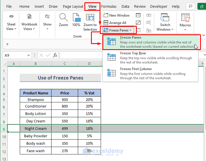
1. Freeze Panes
The Freeze Panes command on the View tab of the ribbon allows locking rows, columns or both. To use:
- Select the cell below the rows you want frozen.
- Go to View > Freeze Panes > Freeze Panes.
- This locks all rows above and columns to the left of the selected cell.
2. Freeze Top Row
To only freeze the first row:
- Go to View > Freeze Panes > Freeze Top Row.
- Just the header row will now stay locked.
3. Split Panes
The Split button separates your sheet into two scrollable panes
- Select the row below where you want to split.
- Click View > Split.
- Rows above split remain frozen.
4. Freeze Using VBA
You can lock rows via VBA code:
-
Select a cell below rows to freeze.
-
Open VBA editor and insert this code:
vbActiveSheet.Range("A4").Select ActiveWindow.FreezePanes = True -
Run the macro to lock rows above selected cell.
5. Format as Table
Format as Table automatically freezes header row:
- Select data range and go to Home > Format as Table.
- The table headers will now remain visible.
6. Keyboard Shortcut
Use the Alt + W + F shortcut to quickly freeze panes.
- Select cell below rows to freeze first.
- Press Alt + W + F to lock rows above selection.
When to Lock Rows in Excel
Here are common cases where you’ll want to freeze rows on an Excel worksheet:
- Locking headers – Keep column labels visible when scrolling through data.
- Freezing filters – Lock drop downs in place on filtered reports.
- Anchoring totals – Fix summation rows to always display on a scrollable report.
- Holding parameters – Freeze lookup values you need to reference while scrolling.
- Retaining titles – Fix top rows that title or headline your worksheet contents.
Locking rows only takes a couple clicks so take advantage of it whenever you need to keep referencing rows visible.
Tips for Freezing Rows in Excel
Follow these tips when freezing rows in your Excel worksheets:
- Freeze the fewest rows needed. Too many locked rows limits scrolling.
- But make sure to freeze enough rows to view labels, filters, etc.
- Freeze columns on the left as well for dual anchoring.
- Format locked rows differently for easy identification.
- Double check frozen rows display correctly before sharing.
- Unfreeze rows if not needed anymore to maximize scrolling.
Unfreezing Rows in Excel
If you need to unfreeze locked rows, simply:
- Go to View > Window > Unfreeze Panes to release all frozen panes.
- Or select a new cell and re-freeze panes to just unlock rows.
Unfreezing clears all locked rows and columns, allowing the full sheet to scroll again.
Troubleshooting Frozen Rows Issues
Here are some common problems when freezing rows and how to fix them:
- Can’t freeze – Make sure you’re not editing a cell. Exit a cell before freezing.
- Freeze not working – The sheet may be protected. Unprotect it first.
- Rows not staying locked – Cells may be inserted/deleted above frozen rows, pushing them down.
- Blank rows appear – Rows hidden before freezing become visible when locked.
Carefully check for these issues if freezing rows isn’t working as expected.
Using Excel Tables to Lock Rows
Formatting your data as an Excel Table is another great way to freeze header rows. Just:
- Select your data cells and go to Home > Format as Table.
- In the dialog, check “My table has headers”.
- The header row will now stay locked in place.
Tables also give your data some other great benefits like structured references and auto-expanding ranges.
VBA Code for Freezing Rows
In addition to the manual steps above, you can use VBA macros to freeze rows in Excel.
For example, this short code locks rows based on a target cell:
Sub FreezeRows() Range("A3").Select ActiveWindow.FreezePanes = True End SubHere are some key points for freezing via VBA:
- Select a cell below where you want rows frozen before running.
- Set
ActiveWindow.FreezePanes = Trueto lock rows and columns. - Use
ActiveWindow.FreezePanes = Falseto unfreeze rows.
Macros let you quickly freeze rows without navigating through the menus.
Dynamic Freezing with Offset
You can even write a macro to dynamically freeze rows based on the last row with data rather than a fixed row number:
Dim lastRow As LonglastRow = Cells(Rows.Count, "A").End(xlUp).RowRange("A3").Offset(lastRow - 3, 0).SelectActiveWindow.FreezePanes = TrueThis finds the last used row, offsets to freeze below it, and sets freeze panes there.
Key Takeaways
The ability to lock rows in Excel provides important visibility and reference points when scrolling large worksheets. Here are some key things to remember:
- Use Freeze Panes, Split, and other options to lock header and data rows.
- Format as Table also freezes the header row automatically.
- Unfreeze panes when you no longer need rows locked.
- Write VBA macros to freeze rows on the fly with shortcuts.
- Offset formulas can dynamically set freeze rows based on data.
Locking rows takes just seconds but pays dividends by anchoring your most important Excel data in place!
Excel Freeze Top Row and First Column (2020) – 1 MINUTE
How do I lock multiple rows in Excel?
Freeze Panes – to lock several rows. The detailed guidelines follow below. To lock top row in Excel, go to the View tab, Window group, and click Freeze Panes > Freeze Top Row. This will lock the very first row in your worksheet so that it remains visible when you navigate through the rest of your worksheet.
How do I freeze a row in Excel?
If you want the row and column headers always visible when you scroll through your worksheet, you can lock the top row and/or first column. Tap View > Freeze Panes, and then tap the option you need. Select the row below the last row you want to freeze. On your iPad, tap View > Freeze Panes > Freeze Panes.
How do I lock the top 5 rows in Excel?
Let’s assume you want to lock the top five rows. Follow these steps: Select cell A6 or the row header for row 6. Select View, Freeze Panes, and then the Freeze Panes option in the drop-down. The top five rows won’t move when you scroll down.
How do I lock a row in Windows 10?
Step 1: Navigate to the View tab and locate the Window group. Step 2: Click Freeze Panes and select Freeze Top Row from the drop-down menu. This will lock only the top row. You can see a black line under the first row which signals that the row is now locked. If you are looking to lock multiple rows, follow these instructions:
