The tutorial explains the process of making a line graph in Excel step-by-step and shows how to customize and improve it.
The line graph is one of the simplest and easiest-to-make charts in Excel. However, being simple does not mean being worthless. As the great artist Leonardo da Vinci said, “Simplicity is the greatest form of sophistication.” Line graphs are very popular in statistics and science because they show trends clearly and are easy to plot.
So, lets take a look at how to make a line chart in Excel, when it is especially effective, and how it can help you in understanding complex data sets.
A line chart is a popular graphical tool used to visualize trends and patterns in data over a period of time. With a line chart, you can see the fluctuations and progression of numeric values clearly.
In this comprehensive guide, I will walk you through the steps to insert a simple line chart as well as a multi-line chart in Excel. I will also share tips to customize your line chart to make it look polished and professional.
When to Use a Line Chart
A line chart is best suited for
-
Visualizing data and trends over a continuous period of time. The ups and downs in the line show increases and decreases in values.
-
Comparing multiple data series side-by-side. Multi-line charts allow you to contrast trends.
-
Showing progression You can assess progress towards a goal with a line chart
-
Displaying changes over equal intervals of time – like months, quarters, years etc The consistent intervals make trends easy to interpret.
How to Create a Simple Line Chart in Excel
Follow these simple steps to create a basic line chart in Excel:
-
Enter your data – In a spreadsheet, input the data to create your line chart. The x-axis data (dates, months or years) should be in the left column. The y-axis values (numeric data) should be in the columns to the right.
-
Select the data – Highlight the data to be included in the chart. You only need to select one cell – Excel will automatically select the entire data range.
-
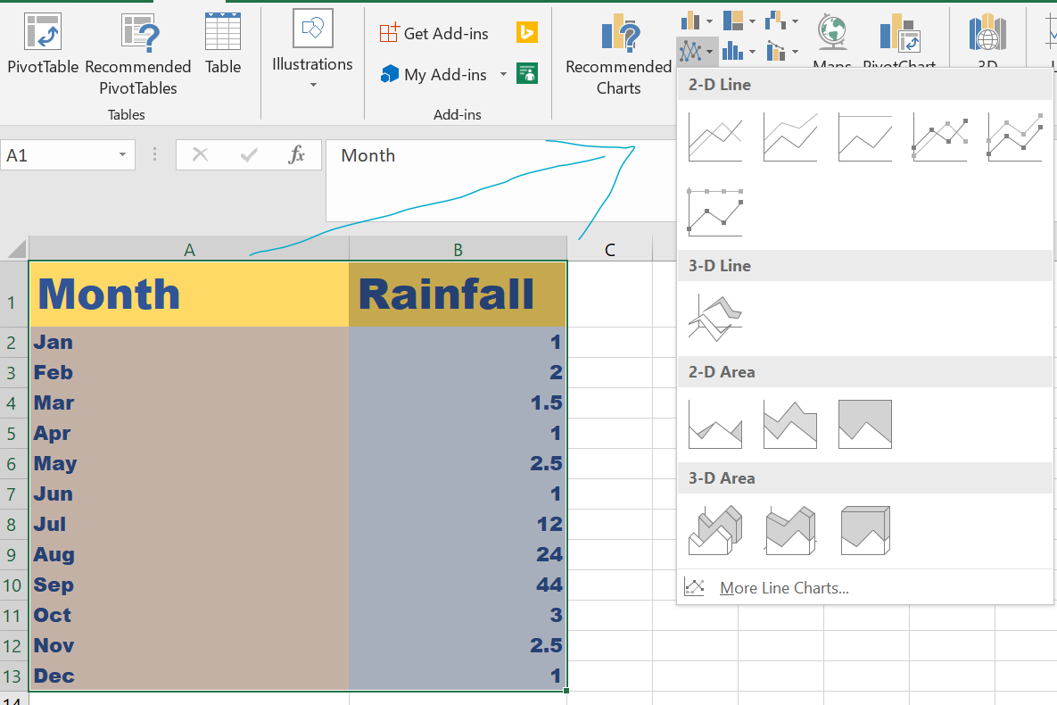
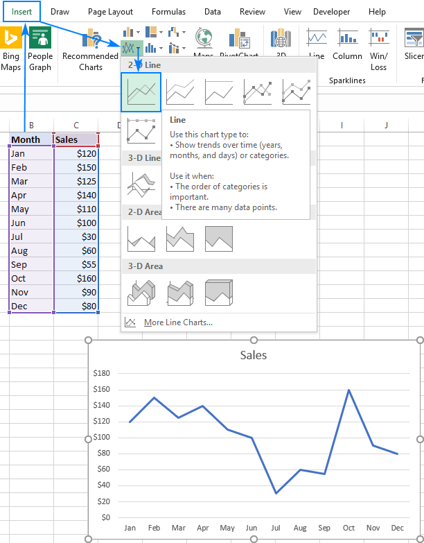
Go to Insert tab – Go to the Insert tab in the Excel ribbon and click on the ‘Line Chart’ icon.
-
Pick a chart style – Hover over different line chart thumbnails and select the style you want.
-
Insert your chart – Click on a chart style to insert it on the worksheet.
And your line chart is ready! The default chart inserted by Excel looks clean and readable. But you can customize it further as needed.
How to Create a Multi-Line Chart in Excel
To compare multiple data series in one chart, you can create a multi-line chart. The steps are mostly the same:
-
Enter data with x-axis values in the first column and y-axis values for each data series in subsequent columns.
-
Highlight the entire data range, including headers.
-
Go to Insert -> Line Chart. Pick a multi-line chart style like ‘Line with Markers’.
-
Insert the chart in the sheet.
With a few clicks, you will have a multi-line chart to contrast trends! Make sure to limit the number of lines between 3-4 for better readability.
Customizing Your Excel Line Chart
Don’t stop at the basic line chart inserted by Excel. Make your chart stand out by customizing it proficiently. Here are some useful ways to enhance your line chart:
-
Add a meaningful title – Summarize the key message of your chart with a title. Go to Chart Tools -> Layout tab to add and format it.
-
Include informative axis labels – Replace the default axis titles with ones that are concise. Go to Format Axis option.
-
Adjust scale of axes – Change the scale or units on the axes to best represent your data range. Use Format Axis.
-
Show or hide gridlines – Gridlines make it easier to read values. Toggle them on or off from the Format tab.
-
Change chart style and colors – Modify overall style, color scheme and theme from Design and Format tabs.
-
Add a legend – Use a legend to help distinguish multiple lines. Position it smartly so it doesn’t overlap data.
-
Add data labels – Data labels show values next to data points for context. Enable them from Layout tab.
-
Include source data – Add a data table to show the spreadsheet data alongside the chart. Use Layout tab.
-
Smooth jagged lines – For a sleeker look, you can smooth jagged lines. Double click the line and check ‘Smoothed line’ option.
-
Add trendline – Insert linear or exponential trendlines to show overall trends. Access from the ‘+’ button.
With the right customizations, your Excel line chart can look highly polished, professional and convey information effectively!
Helpful Tips for Better Line Charts
Here are some useful tips to improve your Excel line charts:
-
Limit the number of data points to under 50. Too many data points make the chart overly crowded.
-
Label the axes, title and legend accurately to make the chart self-explanatory.
-
Use different line styles, widths and markers to distinguish overlapping lines.
-
Show only essential chart elements. Clutter obscures the key message.
-
Use background color, borders and effects to make key lines stand out.
-
Keep variations in y-axis values moderate. Very high peaks distort trends.
-
Add forecast trendlines if useful to show projections.
-
Maintain 3:2 length-to-height ratio for line chart shape. Square charts look cramped.
Common Problems in Line Charts
Here are some frequent issues in Excel line charts and ways to fix them:
-
Overlapping lines make it hard to differentiate series – use different colors, dashes, markers.
-
Gaps in lines – check for blank cells in data range and fill them.
-
Missing data points – verify source data range. Expand range if needed.
-
Jumbled x-axis labels – check if data is sorted properly and chronologically.
-
Very high or low values distort scale – change axis bounds manually to normalize.
-
Flattened peaks/troughs – decrease gap width to expand horizontal axis scale.
Examples of Good Excel Line Charts
Here are two examples of clean, effective line charts created in Excel:
<div style=”text-align:center”><img src=”https://i.imgur.com/nYRlJ2J.png” alt=”Sales Growth Line Chart”></div><div style=”text-align:center”><img src=”https://i.imgur.com/F0eGWaS.png” alt=”Multi-line Chart”></div>
Change data markers in a line graph
When creating a line chart with markers, Excel uses the default Circle marker type, which in my humble opinion is the best choice. If this marker option does not fit well with the design of your graph, you are free to choose another one:
- In your graph, double-click on the line. This will select the line and open the Format Data Series pane on the right side of the Excel window.
- On the Format Data Series pane, switch to the Fill & Line tab, click Marker, expand Marker Options, select the Built-in radio button, and choose the desired marker type in the Type box.
- Optionally, make the markers larger or smaller by using the Size box.
How to make a line graph in Excel
To create a line graph in Excel 2016, 2013, 2010 and earlier versions, please follow these steps:
- Set up your data A line graph requires two axes, so your table should contain at least two columns: the time intervals in the leftmost column and the dependent values in the right column(s). In this example, we are going to do a single line graph, so our sample data set has the following two columns:

- Select the data to be included in the chart In most situations, it is sufficient to select just one cell for Excel to pick the whole table automatically. If youd like to plot only part of your data, select that part and be sure to include the column headers in the selection.
- Insert a line graph With the source data selected, go to the Insert tab > Charts group, click the Insert Line or Area Chart icon and choose one of the available graph types. As you hover the mouse pointer over a chart template, Excel will show you a description of that chart as well as its preview. To inset the chosen chart type in your worksheet, simply click its template. In the screenshot below, we are inserting the 2-D Line graph:
 Basically, your Excel line graph is ready, and you can stop at this point… unless you want to do some customizations to make it look more stylish and attractive.
How to Make a Line Graph in Excel
How to insert line chart in Excel?
Step 1: To insert line chart in Excel, select the cells from A2 to E6. Go to the Insert tab, and choose the “ Insert Line or Area Chart ” option in the Charts group. Choose any line chart; here, we choose the “Line with Markers” option. You get a graph as shown below.
How do I use a single line graph in Excel?
We will now use a basic line graph to represent this data. For that: Select data in both columns. Click Recommended Charts on the Charts group. An Insert Chart dialog box will appear. Select the chart type you want to use. For now, we will use a single-line graph.
How to draw a line graph in Excel?
Go to the Insert tab > Charts group and click Recommended Charts. Done! A horizontal line is plotted in the graph and you can now see what the average value looks like relative to your data set: In a similar fashion, you can draw an average line in a line graph.
How to create a 3D line chart in Excel?
Step 1: To plot the graph, select the data in the table from cells A2 to C6. Go to the “ Insert ” menu. In the “ Charts ” Tab, click on the “ Insert Line or Area Chart ” symbol. From here, we can select a required line chart. Here, we choose the 3-D line chart.
