The tutorial shows different ways to insert an in Excel worksheet, fit a picture in a cell, add it to a comment, header or footer. It also explains how to copy, move, resize or replace an in Excel.
While Microsoft Excel is primarily used as a calculation program, in some situations you may want to store pictures along with data and associate an with a particular piece of information. For example, a sales manager setting up a spreadsheet of products may want to include an extra column with product s, a real estate professional may wish to add pictures of different buildings, and a florist would definitely want to have photos of flowers in their Excel database.
In this tutorial, we will look at how to insert in Excel from your computer, OneDrive or from the web, and how to embed a picture into a cell so that it adjusts and moves with the cell when the cell is resized, copied or moved. The below techniques work in all versions of Excel 2010 – Excel 365.
Adding images and pictures into your Excel workbooks can make them much more visually engaging and easy to understand
In the past, it was only possible to place images over cells in Excel. This would cover up data and make it hard to interact with the cells underneath.
Fortunately, Excel now has features that allow you to insert pictures directly inside cells while still being able to access the cell data
In this comprehensive guide, you’ll learn multiple methods for getting images into Excel cells. Follow along to start enhancing your spreadsheets with eye-catching visuals.
Why Use Images in Excel?
Before we dig into the how-to, let’s look at some of the benefits of using pictures in Excel:
-
Communicate more effectively – A picture is worth a thousand words. Images allow you to convey information and context faster.
-
Make data more memorable – Research shows we recall information better when text is paired with relevant imagery.
-
Highlight trends or findings – Use representative pictures to underscore notable data points.
-
Add visual appeal – Plain spreadsheets can seem boring. Images make things more lively and engaging.
-
Enhance reports or dashboards – Pictures work nicely alongside Excel charts to visualize data-driven narratives.
Now let’s look at a few different ways you can leverage images inside your Excel files.
Insert Images Using Excel Data Types
A quick and easy way to get images into cells is using Excel’s Data Types feature. Here’s how it works:
-
Select the text cells you want to convert into a data type. This needs to be a predefined geography or financial data type like country, city, stock ticker, etc.
-
On the Data tab, click the data type matching your text, like “Geography”.
-
This converts the cells into data types. Click the map icon to view the data card with more details.
-
Select the data type cells and click “Extract” > “Image” from the ribbon to pull the images into adjacent cells.
The Geography data type works great for inserting flag images of countries, states, cities, etc. The Stocks data type contains company logo images you can extract.
While simple, the downside is you can’t insert custom images – just those predefined by the data type.
Use Organization Data Types for Custom Images
If you want to insert your own images into cells, you can build custom Organization data types using Power BI. Here’s how:
-
Import your image URLs list into Power BI Desktop and load it as a table.
-
Mark the table as Featured and set a Row Label column along with Image URL and Key columns.
-
Publish this as a dataset to your Power BI workspace.
-
In Excel, convert your Row Label text into the new Organization data type.
-
Extract the image using “Data Type Cell Name.Image” just like with built-in data types.
This takes more setup but allows you to use your own images in Excel. Just be sure to set up the data model correctly in Power BI.
Insert Any Image with the IMAGE Function
The most flexible way to add images to cells is directly through Excel formulas using the IMAGE function.
The IMAGE function inserts pictures based on a valid image URL. For example:
=IMAGE("https://example.com/image.jpg")The IMAGE function takes these arguments:
-
URL – Path to the image file online. Can be hardcoded or reference a cell with the URL.
-
Alt text (optional) – Text description of the image for accessibility.
-
Sizing option (optional) – How to fit the image in the cell.
With IMAGE, you can insert any openly accessible image on the web into a cell with a simple formula.
Step-by-Step Guide to Inserting Images in Cells
Follow along as we walk through an example of adding product images to an inventory spreadsheet using the IMAGE function.
Set Up the Spreadsheet
First, we’ll add a table to the spreadsheet with product names, IDs, and image URLs:
<img src=”https://example.com/image1.png” width=”300px” alt=”Table with columns for product name, ID, and image URL”>
The image URLs point to product photos stored online.
Next, we need a place to display the images. In column E, we’ll add this formula that references the image URL cell:
=IMAGE(C2)This inserts the image for the first row. We’ll fill down this formula to add all product images.
Update Formula Cell References
When filling the formula down, we need to update the cell references. Double click the bottom right corner of cell E2 to fill down the column and automatically update the URLs:
<img src=”https://example.com/image2.png” width=”300px” alt=”Column filled down with updated cell references”>
Now the formula references each row’s unique image URL.
Set Image Sizing and Alt Text
The images may be too large or small for the cells. To resize, add the optional sizing argument:
=IMAGE(C2,,"1")The ,, skips the alt text parameter to just include the sizing argument. Setting it to 1 sizes the image to fill the cell.
For accessibility, let’s also add the alt text parameter:
=IMAGE(C2,"Product image","1")Now image sizing and alt text are set.
Final Spreadsheet
Here is the final spreadsheet with images inserted in the cells successfully:
<img src=”https://example.com/image3.png” width=”500px” alt=”Final spreadsheet with images inserted into cells”>
The IMAGE function allows us to dynamically pull images into the Excel grid based on URLs in another column.
Tips for Using Images in Cells
Here are some best practices for working with images inside Excel cells:
-
Store images online so you have permanent URLs to reference.
-
Make image URLs public or accessible to anyone with the link for the IMAGE formula to work.
-
Set alt text for all images to describe them for screen reader accessibility.
-
Adjust image sizing and cell width/height to avoid distorted images.
-
Link images to source cells so they update automatically if you move cells around.
Next Steps for Enhancing Excel Visuals
Adding simple images is just one step to take your spreadsheets to the next level. Also consider:
-
Infographics – Use SmartArt and shapes to visualize data trends.
-
Charts – Insert clustered columns, line charts, or other graph types to make data interactive.
-
Sparklines – Include tiny charts in cells to show data changes.
-
Icons – Supplement text with explanatory icons and emoji.
With the power to now place images inside cells, you can make your Excel reports, dashboards, trackers, and models far more engaging and effective.
Images allow you to convey more information through visuals that quickly grab attention while also improving comprehension and recall.
Use the techniques covered in this guide to start incorporating images into your Excel spreadsheet data for maximum visual impact.
How to insert multiple pictures into cells in Excel
As you have just seen, its quite easy to add a picture in an Excel cell. But what if you have a dozen different s to insert? Changing the properties of each picture individually would be a waste of time. With our Ultimate Suite for Excel, you can have the job done in seconds.
- Select the left top cell of the range where you want to insert pictures.
- On the Excel ribbon, go to the Ablebits Tools tab > Utilities group, and click the Insert Picture button.
- Choose whether you want to arrange pictures vertically in a column or horizontally in a row, and then specify how you want to fit s:
- Fit to Cell – resize each picture to fit the size of a cell.
- Fit to – adjust each cell to the size of a picture.
- Specify Height – resize the picture to a specific height.
- Select the pictures you want to insert and click the Open button.
Note. For pictures inserted in this way, the Move but dont size with cells option is selected, meaning the pictures will keep their size when you move or copy cells.
Inserting an into an Excel comment may often convey your point better. To have it done, please follow these steps:
- Create a new comment in the usual way: by clicking New Comment on the Review tab, or selecting Insert Comment from the right-click menu, or pressing Shift + F2.
- Right click the border of the comment, and choose Format Comment⦠from the context menu. If you are inserting a picture into an existing comment, click Show All Comments on the Review tab, and then right-click the border of the comment of interest.

- In the Format Comment dialog box, switch to the Colors and Lines tab, open the Color drop down list, and click Fill Effects:

- In the Fill Effect dialog box, go to the Picture tab, click the Select Picture button, locate the desired , select it and click Open. This will show the picture preview in the comment. If you want to Lock picture aspect ratio, select the corresponding checkbox like shown in the screenshot below:

- Click OK twice to close both dialogs.
The picture has been embedded into the comment and will show up when you hover over the cell: 
How to resize picture in Excel
The easiest way to resize an in Excel is to select it, and then drag in or out by using the sizing handles. To keep the aspect ratio intact, drag one of the corners of the . 
Another way to resize a picture in Excel is to type the desired height and width in inches in the corresponding boxes on the Picture Tools Format tab, in the Size group. This tab appears on the ribbon as soon as you select the picture. To preserve the aspect ratio, type just one measurement and let Excel change the other automatically. 
How to insert image in excel cell
How to insert a picture in Excel?
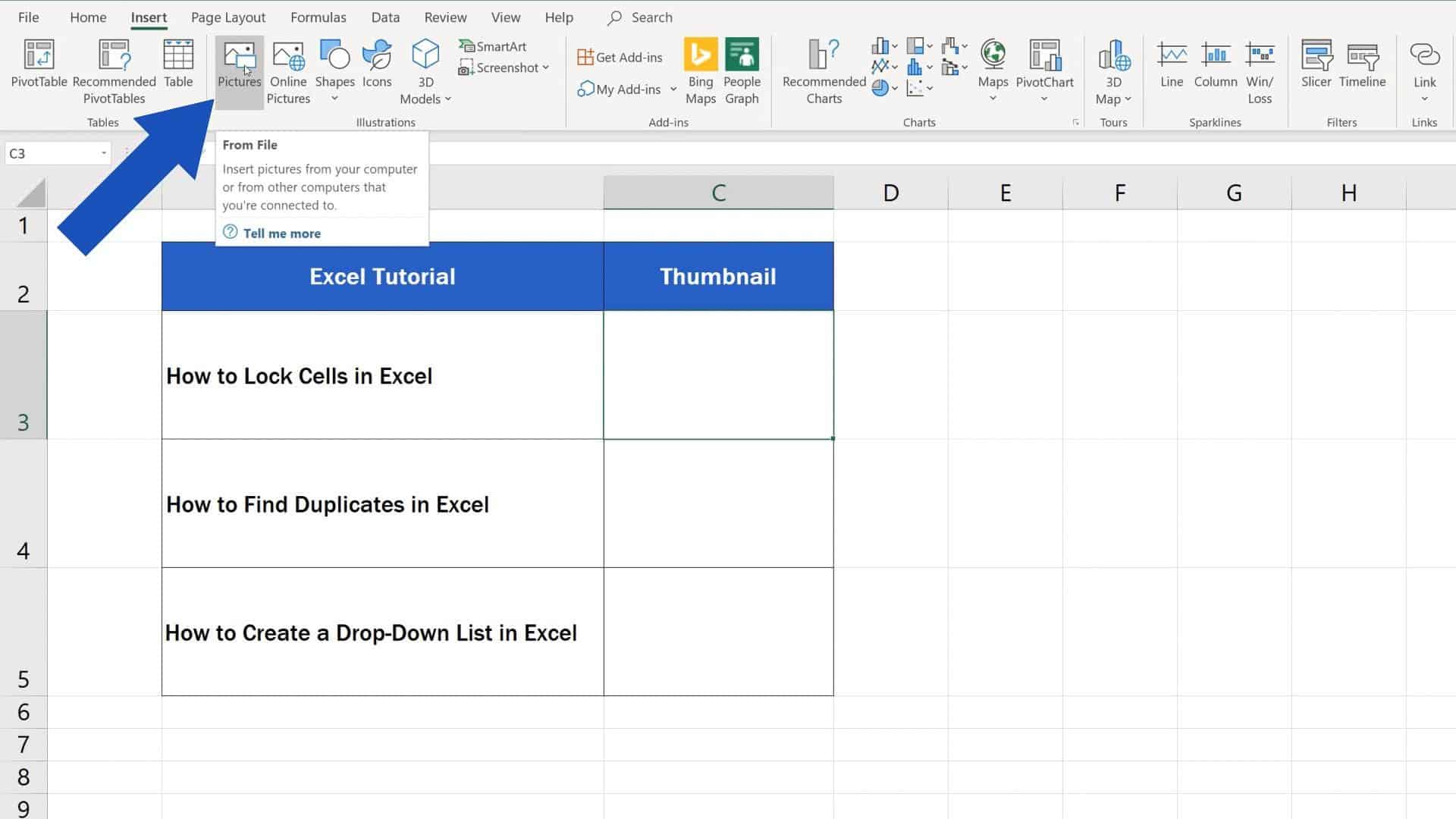
Click the location in your worksheet where you want to insert a picture. On the Insert ribbon, click Pictures. Select Stock Images… Browse to the picture you want to insert, select it, and then click Open. There are numerous approaches you can take in Excel to insert an image.
How to insert and resize images in a cell in Excel?
Let us now first unlock the technique to insert and resize the image in a cell in Excel. Under the excel ribbon options, click on the ‘ Insert ‘ tab and under the ‘ Illustration ‘ group, click on the ‘ Pictures ‘ button. As a result, the ‘ Insert Picture ‘ dialog box would appear on your screen.
How does image work in Excel?
That’s finally changing. Microsoft is now testing a new function in Excel, called IMAGE, which returns an image within a cell. Unlike the existing method of inserting an image (from the Insert tab), the new function keeps the image inside the cell, so it can stay in its intended place as you adjust rows and columns.
