Whenever Im working with large datasets in Google Sheets, its easy for me to lose track of whats what—especially without headers locked in place. Take this simple student grade sheet below, for example.
Notice that as I scroll across the sheet, the student names and IDs disappear. With this view, its nearly impossible for me to remember which grade belongs to which student.
Thats where the Freeze function comes in. It lets you pin columns in place so you can see the data you need at all times, even as you scroll through your spreadsheet.
To get started with a Zap template—what we call our pre-made workflows—just click on the button. It only takes a few minutes to set up. You can read more about setting up Zaps here.
Google Sheets allows you to create powerful spreadsheets for data tracking, analysis, and visualization. But as your sheets grow in size, it can get tricky to navigate and scroll through all the rows and columns. Freezing cells in Google Sheets locks specific rows and columns in place, allowing you to scroll through the rest of the sheet while always keeping those frozen cells visible.
Learning this simple trick can save you tons of frustration Read on as we break down step-by-step how to freeze cells in Google Sheets on desktop and mobile,
Why Freezing Cells is Useful in Google Sheets
Freezing cells creates fixed headers and sidebars that don’t move as you scroll down or across a sheet. This keeps important information like column headers visible as you navigate through data.
Here are some of the most common ways freezing cells can help you in Google Sheets:
- Keep column and row headers in view when scrolling through a large spreadsheet
- Freeze the first column to always view the row labels
- Lock filters or totals columns on the right so they don’t disappear when scrolling horizontally
- Freeze the top row to keep the column labels visible when scrolling down
- Freeze both the first column and first row to lock the labels for both
Freezing is perfect for keeping vital data on screen at all times, like headers, categories, IDs, labels, filters, totals, summaries, or key information you need to reference.
How to Freeze Rows and Columns in Google Sheets
Freezing cells in Google Sheets only takes a couple of clicks. Here is a step-by-step guide to freezing rows and columns in desktop and mobile:
On Desktop
-
Open the Google Sheet and select the cell where you want the freeze to start. This is usually the cell directly below the rows you want frozen and directly right of the columns to freeze.
-
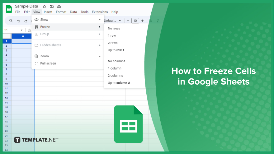
Click View > Freeze from the top menu.
-
Select either Freeze rows or Freeze columns depending on what you want to lock in place.
-
Enter the number of rows or columns you want frozen. For example, freezing 1 row keeps your header locked, and freezing 1 column keeps the first column fixed.
-
The selected rows and columns will now stay fixed on screen as you scroll through the rest of the sheet.
On Mobile
-
In the Google Sheets iOS or Android app, open the sheet and tap the cell below the rows you want to freeze or right of the columns.
-
Tap the expansion menu in the upper-right corner (the 3 dots icon).
-
Choose Freeze rows or Freeze columns.
-
Enter the number of rows or columns to freeze and tap Done.
The steps are the same whether you want to freeze rows, columns, or both. Play around with different freeze settings to find the view that works best for your sheet.
Unfreezing Rows and Columns
Need to unfreeze cells? No problem! Here is how to unfreeze rows and columns when you no longer need them locked in place:
On Desktop
-
Click in any frozen cell and select View > Freeze again from the menu.
-
Choose Unfreeze rows and/or Unfreeze columns.
-
The freeze will be removed, allowing you to scroll freely again.
On Mobile
-
Tap any frozen cell and open the expansion menu.
-
Tap Unfreeze rows or Unfreeze columns.
-
The freeze will be lifted.
Once you unfreeze, all your rows and columns will scroll and operate normally without any fixed sections.
Handy Tips for Freezing Cells in Google Sheets
-
Resize column widths and row heights before freezing cells so the fixed sections appear neatly formatted.
-
Double check that you’ve selected the right freeze cell so the data you want locked is actually fixed in place.
-
Sort and filter your sheet before freezing key columns in place.
-
Format frozen rows and columns with alternate colors to make the fixed sections stand out.
-
Freeze multiple rows or columns as needed to keep all important information visible.
-
Try horizontal and vertical freezes together to fix both column headers and row labels simultaneously.
-
Unfreeze cells when you no longer need certain data to be locked in view.
-
On mobile, tap frozen cells to select them just like any other cell.
-
When inserting/deleting rows or columns, be aware it will push your frozen sections down or to the right.
Advanced Freezing Tips for Google Sheets
Google Sheets offers a few advanced options when freezing cells that can help optimize your view:
Freeze Multiples Sheets Simultaneously
If you have an Excel-style workbook with multiple sheets, you can freeze the same rows and columns across all the sheets at once:
-
Select the tab of the sheet where you want the freeze set.
-
Freeze the desired rows and columns on that sheet.
-
At the bottom, check the Freeze rows and columns on other sheets box.
Now the same freeze will apply to all sheets in your workbook.
Split Freezes
You can also split freezes so, for example, columns 1-3 are frozen while columns 7 onward are frozen, with a scrollable section in between.
To do this:
-
Freeze the first set of columns (1-3 in the example).
-
Scroll to the cell where you want the next freeze to start (column 7).
-
Freeze this column and further ones.
-
The two frozen sets will be locked in place with scrollable columns in between.
Split freezes allow you to fix different sections visible as needed.
Custom Fixed Areas
For maximum control, you can use Data > Protected sheets and ranges to define a custom frozen area that follows your scroll:
-
Select the cells for the range you want to freeze.
-
Go to Data > Protected sheets and ranges.
-
Choose Protect this range and hit Done.
Now your selected range will stay fixed on screen as you scroll, even if it’s not a continuous range of rows or columns.
Wrap Up
Freezing rows and columns takes Google Sheets from messy and unwieldy to clean and usable. Definitely take the time to experiment with different freeze settings and find the right configuration for your spreadsheet.
As your data changes, remember to adjust your frozen areas as needed. Mastering this simple trick will save you tons of aggravation!
How to freeze columns in Google Sheets
Heres the easiest way to freeze a column or multiple columns in Google Sheets.
In the top-left corner of your spreadsheet, next to column A and above row 1, there are two thick, gray bars running horizontally and vertically.

To freeze a column, click the vertical bar and drag it across to the right side of the last column you want to freeze. For example, lets pin up to the student IDs in column C.
To unfreeze a column, drag the bar back to its original position.
If you, like me, get frustrated about having to get your cursor in just the right spot, theres another way.
- Open a Google Sheets spreadsheet.
- Select the columns you want to freeze.
- Click View, and then select Freeze.
- Click Up to column [column letter].
Lets freeze the student IDs in column C again using this method. For this example, click View, select Freeze, and select Up to column C.

Its a simple example, but when youre reviewing grades for 30 or so students—or youre working with a large dataset of any sort—freezing columns and rows makes scrolling through the data much more manageable.
To unfreeze a column, repeat the same steps, but instead of clicking Up to column C, click No columns.
Manual data entry is ripe for human error. With Zapier, you can connect Google Sheets with your go-to apps. This way, you can automate your most time-consuming spreadsheet-related tasks. For example, you can automatically add new lead data and form submissions to an existing spreadsheet. Learn more about how to automate Google Sheets, or get started with one of these workflow templates.
To get started with a Zap template—what we call our pre-made workflows—just click on the button. It only takes a few minutes to set up. You can read more about setting up Zaps here.
Related reading:
How to Freeze Multiple Rows and or Columns in Google Sheets using Freeze Panes
How do I freeze a spreadsheet?
You can freeze, group, hide, or merge your spreadsheet’s columns, rows, or cells. To pin data in the same place and see it when you scroll, you can freeze rows or columns. On your computer, open a spreadsheet in Google Sheets. Select a row or column you want to freeze or unfreeze. At the top, click View Freeze.
How do I freeze a spreadsheet in Google Sheets?
On the top left-hand corner of your Google Sheets spreadsheet, you will find both a vertical and horizontal gray pane as shown below. When you hover your mouse over those gray-colored panes, it turns into a hand icon. Simply drag each pane either vertically or horizontally until they sit below the columns or rows you wish to freeze.
How to freeze rows in Google Sheets?
Freezing up to two rows can be done using the predefined options. However, if you wish to freeze any row beyond the second one, make sure to select the proper cell and then choose the fourth option, as discussed above. This is the last method to freeze rows in Google Sheets.
What happens if you freeze a column in Google Sheets?
If you freeze columns or rows in Google Sheets, it locks them into place. This is a good option for use with data-heavy spreadsheets, where you can freeze header rows or columns to make it easier to read your data. In most cases, you’ll want to freeze only the first row or column, but you can freeze rows or columns immediately after the first.
