Calculating differences between values is one of the most common tasks in Excel. Whether you’re analyzing sales data, financial reports, sports statistics or any other type of data, you’ll likely need to find differences to spot trends and make comparisons.
In this comprehensive guide, I’ll show you multiple methods to calculate differences in Excel, using both simple formulas and powerful functions. By the end, you’ll have a clear understanding of how to find differences in Excel to suit any situation.
Let’s get started!
Why Finding Differences in Excel is Important
Here are some key reasons why calculating differences is an essential Excel skill
-
Spot Trends Over Time By finding differences between values over different periods you can identify rising or falling trends in your data. This helps with forecasting and predicting future numbers.
-
Compare Categories: Subtracting values across different categories reveals how one category performs compared to another. For example, you can compare sales by region.
-
Track Changes: Taking the difference between two versions of data shows exactly how and where values have changed. Useful for financial reports and auditing.
-
Calculate Metrics: Many key performance metrics rely on finding differences. For example, percentage change, growth rate and delta are based on subtracting old and new values.
As you can see, regularly calculating differences provides vital insights into your data. Let’s look at the various ways to do this in Excel.
Method 1: Simple Subtraction Formula
The most straightforward way to find the difference between two values is to simply subtract one from the other using the minus formula.
Here is the structure:
=Value1 – Value2
Where Value1 is the value you’re subtracting from and Value2 is the value you’re subtracting.
For example, to find the difference between the numbers in cells A2 and B2, use this formula:
=A2-B2
When you hit Enter, Excel performs the subtraction and returns the difference.
Let’s see a full example:
![Subtraction Example][]
Here we have sales data for two months. To calculate the difference between Jan and Feb sales, we input the formula =B2-C2 in cell D2. Excel computes the subtraction and shows that Feb sales were $530 higher than Jan sales.
You can use this method for both numbers and time values. Just make sure the values you’re subtracting have compatible formats, i.e. both are numbers or both are times/dates.
Pro Tip: You can also subtract entire columns or rows using this method. For example, to get the differences between values in Column A and Column B, use this formula in Column C:
=A1-B1
And fill down for all rows. This subtracts each row of B from the corresponding row in Column A.
Method 2: The MINUS Function
While the simple minus formula works fine, Excel also provides the MINUS function which is specially designed for subtraction.
The MINUS function takes two inputs:
=MINUS(Value1, Value2)
Value1 is the minuend (the number you are subtracting from) and Value2 is the subtrahend (the number you are subtracting).
For example, to subtract B2 from A2:
=MINUS(A2,B2)
This function performs exactly the same subtraction as the minus formula. So you may be wondering – why use MINUS at all?
Here are two advantages of the MINUS function:
- Formula Auto-Updating: If the referenced values change, MINUS will automatically recalculate, while regular formulas won’t update unless you press F9.
- Formula Clarity: MINUS makes your intention clearer when reading the formula.
So in some cases, MINUS is preferable over the basic minus formula.
Method 3: The DIFFERENCE Function
Another way to calculate differences in Excel is with the DIFFERENCE function.
The syntax is:
=DIFFERENCE(Value1, Value2)
It works the same as MINUS – Value1 is the number you subtract from and Value2 is the number you subtract.
For example:
=DIFFERENCE(A2,B2)
Subtracts the value in B2 from A2.
DIFFERENCE and MINUS produce identical results. DIFFERENCE is simply an alternative name for the subtraction operation.
So MINUS and DIFFERENCE can be used interchangeably based on your preference.
Method 4: The ABS Function
When taking differences, you sometimes only care about the absolute value or magnitude of the difference, not whether it’s positive or negative.
That’s where the ABS (absolute) function comes in handy.
ABS returns the absolute value of a number, removing any negative sign while keeping positives unchanged.
To use ABS for difference calculation, wrap it around a regular subtraction formula:
=ABS(Value1-Value2)
This finds the difference between Value1 and Value2, then makes the result an absolute positive number.
For example:
=ABS(A2-B2)
Subtracts B2 from A2 and converts the result to a positive value.

Here, the profit in Cell B4 is negative while A4 is positive. Taking the regular difference would result in a larger negative number.
But with ABS, it takes the difference and flips the negative to a positive, giving us the magnitude of profit change.
Method 5: Percentage Difference
While subtracting two values directly can be useful, often you need to express the difference in percentage terms compared to the original values.
Calculating percentage difference helps you analyze changes in relative rather than absolute terms.
Here is the formula for percentage difference in Excel:
=(New Value – Original Value)/Original Value
To make it a percentage, multiply it by 100:
=((New Value – Original Value)/Original Value)*100
For example, if A2 contains 500 and B2 contains 450, the percentage difference is:
=((B2-A2)/A2)*100
Which gives -10% after calculation.
Let’s look at an example:

Cell C2 uses the percentage difference formula to calculate the percentage change in monthly revenue.
We can see revenue decreased by 5.26% between Jan and Feb. Expressing the difference as a percentage helps better understand the extent of change.
Pro Tip: To calculate percentage increase instead of decrease, swap the order of values so the new value comes first:
=((New Value – Original Value)/Original Value)*100
Method 6: Percentage Change
Closely related to percentage difference is percentage change. While they sound similar, percentage change is calculated differently.
The formula for percentage change is:
=(New Value – Original Value) / Absolute(Original Value)
It divides the difference by the absolute original value, not just the original value.
For example, if A2 is 500 and B2 is 450, the percentage change is:
=(B2-A2)/ABS(A2)
Which gives -10% after calculation.
Here’s an example showing both percentage difference and percentage change:

You can see percentage change gives a different value than percentage difference.
Use percentage difference when you want to compare two values directly. Use percentage change when measuring growth or reduction.
Method 7: Average Difference
When comparing two sets of data, you may want to know the average or mean difference between the sets.
For example, average differences in sales, profits or temperatures.
Here is the formula for average difference in Excel:
=AVERAGE(Set1 – Set2)
Where Set1 and Set2 are the two data sets you want to compare.
For example, if you have sales data for 2021 in A2:A11 and 2022 in B2:B11, the average difference is:
=AVERAGE(A2:A11-B2:B11)
This subtracts each value in Set2 from the corresponding value in Set1, then takes the average of the differences.
Let’s see an example:

We calculate the mean monthly difference in sales between 2021 and 2022. The average sales were $52k higher in 2022.
Finding average differences summarizes disparities between data sets into a single value.
Method 8: Rolling Differences
When analyzing time series data, you may want to calculate the difference between a value and the previous value. This shows how the numbers change over time.
For example, the difference in sales Month-over-Month or Week-over-Week.
Using a Separate Column
In column C, enter the ff. formula into the first cell and then copy it down.
In column D, enter the ff. formula into the first cell and then copy it down.
Both of these should help you visualize which items are missing from the other column.
Microsoft has an article detailing how to find duplicates in two columns. It can be changed easily enough to find unique items in each column.
For example if you want Col C to show entries unique to Col A, and Col D to show entries unique to Col B:
Heres the formula that you are looking for:
Say you want to find those in col. B with no match in col. A. Put in C2:
This will give you 1 (or more) if theres a match, 0 otherwise.
You can also sort both columns individually, then select both, Goto Special, select Row Differences. But that will stop working after the first new item, and you will have to insert a cell then start again.
If I understand your question well:
Replace True/false directives by a function or by a string like “Equal” or “different”.
It depends on the format of your cells and your functional requirements. With a leading “0” they could be formatted as text.
Then you could use IF function to compare cells in Excel:
Example:
If they are formatted as numbers, you could subtract the first column from the other in order to get the difference:
This formula will directly compare two cells. If they are the same, it will print True, if one difference exists, it will print False. This formula will not print what the differences are.
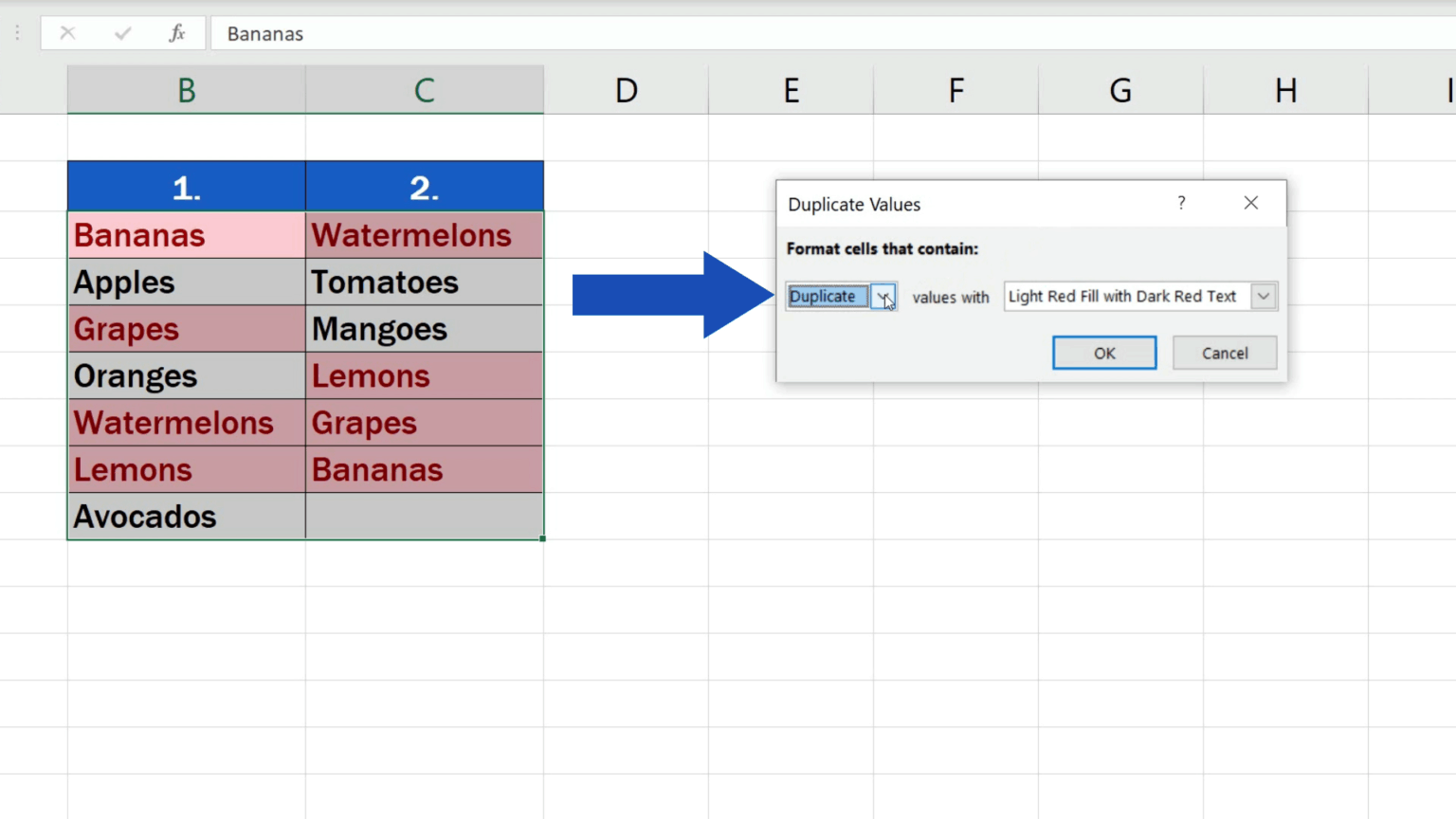
Im using Excel 2010 and just highlight the two columns that have the two sets of values Im comparing, and then click the Conditional formatting dropdown on the home page of Excel, choose the Highlight Cells rules, and then differences. It then prompts to highlight either differences or similarities and asks what colour highlight you want to use…
The comparing can be done with Excel VBA code. The compare process can be made with the Excel VBA Worksheet.Countif function.
Two columns on different worksheets were compared in this template. It found different results as an entire row was copied to the second worksheet.
Code:
This is using another tool but Ive just found this very easy to do. Using Notepad++:
In Excel make sure your 2 columns are sorted in the same order, then copy and paste your columns into 2 new text files and then run a compare (from plugins menu).
The NOT MATCH function combination works well. The following works too:
=IF(ISERROR(VLOOKUP(<
REMEMBER: the smaller list MUST be SORTED ASCENDING – a requirement of vlookup
11 Answers 11 Sorted by:
Highlight column A. Click Conditional Formatting > Create New Rule > Use this formula to determine which cells to format > Enter the ff. formula:
Click the Format button and change the Font color to something you like.
Repeat the same for column B, except use this formula and try another font color.
