I want to highlight/color code the Cell in Column B, based on the value of cell in Column A
On the Home tab of the ribbon, click Conditional Formatting > New Rule… Select Use a formula to determine which cells to format. Enter the formula
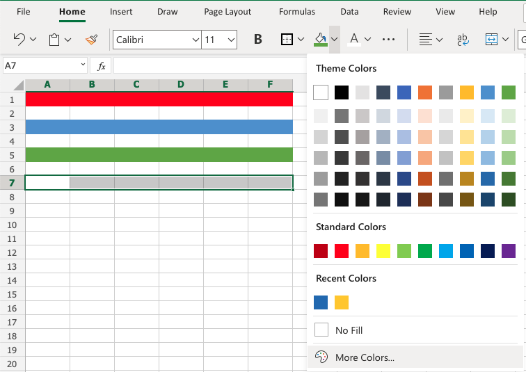
Click Format… Activate the Fill tab. Select red as fill color. Click OK, then click OK again.
However, I have a unique issue at hand. There is an offset in the A and B Columns.
When you select the range in column B to color, the active cell in the selected range should be the first (topmost) cell in that range.
And the formulas in the conditional formatting rules should refer to the cell in that row.
So in this example, the formulas should be =$A6<0 and $A6>0 since the active cell is in row 6.
However, I have a unique issue at hand. There is an offset in the A and B Columns.
Color coding your Excel spreadsheets can make your data pop visually and help viewers quickly absorb key information. Whether you want to highlight values over a threshold differentiate categories or visualize patterns, Excel provides easy ways to add color formatting.
In this beginner’s guide, we’ll walk through the basics of applying color coding in Excel using conditional formatting. Follow along to learn how to
- Use preset color scales and data bars
- Make a single color format based on values
- Apply multiple color formats by rules
- Color code text and cell backgrounds
- Modify and extend color formats
Let’s jump in and add some color to your spreadsheets!
Getting Started with Color Coding
Before applying color formats, you’ll first need data entered in an Excel sheet. Once your sheet is populated, select the cells you wish to color code. This can be a single column, row, or a larger range.
Next, go to the Home tab and click Conditional Formatting. This will open a menu with different formatting types.
Using Preset Color Scales
For a quick color code, try the preset formatting options:
Data Bars
Data bars automatically fill selected cells with horizontal bars shaded from light to dark based on the values. The higher the number, the darker the bar.
Color Scales
Color scales shade the cells with a color gradient from low (red) to mid (yellow) to high values (green).
Both options provide an instant color code without any setup. Just select your data and apply the format.
Single Color Format by Value
To color code your own value thresholds, select New Rule and go to Format only cells that contain. You can pick options like:
- Greater than
- Less than
- Between
- Equal to
- Text that contains
- A date occurring
Enter the threshold value(s) and pick a fill color. This will instantly format cells that meet your rule.
Color Coding by Multiple Rules
Things get more flexible with the New Rule option for “Format all cells based on their values.”
Here you can define multiple color coded ranges in one format. For example:
- Greater than 100 = Green
- 50 to 100 = Yellow
- Less than 50 = Red
Add rules for each range and color. Excel will apply the formats sequentially down your data.
Color Fill vs Font Color
So far we’ve changed the cell fill color, but you can also apply color formats to the text. Simply check “Text color” instead of “Fill” when defining value rules.
Use fill colors to shade the background and font colors to change the text.
Modifying and Extending Color Formats
Once created, conditional formats can be edited by selecting Manage Rules on the Conditional Formatting menu. Here you can tweak value thresholds, colors, and formatting rules.
To apply an existing color format to new data, just select the cells and go to Manage Rules to copy the format over. No need to recreate it!
Examples and Uses for Color Coding
Now that you know the basics, let’s look at some examples of color coding in action:
Color Coded Heat Map
Use a red-yellow-green color scale to visualize data ranges at a glance, like this sales KPI heat map:
<table> <tr> <th></th> <th>Q1 Sales</th> <th>Q2 Sales</th> <th>Q3 Sales</th> <th>Q4 Sales</th> </tr> <tr> <td>West Region</td> <td style=”background-color:green”>$110,000</td> <td style=”background-color:yellow”>$80,000</td> <td style=”background-color:red”>$50,000</td> <td style=”background-color:yellow”>$70,000</td> </tr> <tr> <td>East Region</td> <td style=”background-color:yellow”>$70,000</td> <td style=”background-color:green”>$90,000</td> <td style=”background-color:yellow”>$75,000</td> <td style=”background-color:red”>$45,000</td> </tr></table>
Category Color Coding
Use different colors to distinguish qualitative data like product categories:
<table> <tr> <th>Product</th> <th>Category</th> <th>Price</th> </tr> <tr> <td>Widget Pro</td> <td style=”background-color:blue;color:white”>Hardware</td> <td>$99</td> </tr> <tr> <td>SoftApp</td> <td style=”background-color:orange”>Software</td> <td>$59</td> </tr></table>
Overdue Projects in Red
Emphasize late projects by color coding due dates that have passed:
<table> <tr> <th>Project</th> <th>Due Date</th> <th>Status</th> </tr> <tr> <td>Website Redesign</td> <td>1/15/2022</td> <td style=”background-color:red;color:white”>Overdue</td> </tr> <tr> <td>Brochure Design</td> <td>2/28/2022</td> <td>Upcoming</td> </tr></table>
Opposite Cell Highlighting
Use complementary colors to highlight min/max cells:
<table> <tr> <th>Month</th> <th>Revenue</th> </tr> <tr> <td>January</td> <td style=”background-color:green;color:white”>$250,000</td> </tr> <tr> <td>February</td> <td>$200,000</td> </tr> <tr> <td>March</td> <td>$150,000</td> </tr> <tr> <td style=”background-color:red;color:white”>April</td> <td style=”background-color:red;color:white”>$100,000</td> </tr></table>
Limitations to Keep in Mind
While color coding adds visual pop, be mindful that:
- 10-12 colors is optimal – too many becomes difficult to interpret
- Colors won’t show on black/white printouts
- People with color blindness may have difficulty distinguishing some hues
- Don’t rely solely on color to convey meaning
Use colors to supplement and enhance (not replace) the actual data. Include legends to define your color system when needed.
Quick Recap
That wraps up this beginner’s guide to color coding in Excel using conditional formatting. Here are the key takeaways:
- Use preset options like data bars and color scales for quick formatting
- Make value-based rules to color code your own thresholds
- Apply colors to fills, text, or both
- Modify and extend existing color formats
- Visualize trends, highlight outliers, and categorize data
- Keep accessibility in mind when choosing color schemes
Color coding makes it easier to visualize patterns in your Excel data. With conditional formatting, it’s simple to set up and experiment with different color options.
Now get ready to make your spreadsheets more engaging and easy to parse! Just don’t go overboard with a rainbow of colors.
Related Discussions View all
by erictmtl on February 14, 2024
by jpowell1080 on February 21, 2020
How to Automatically Color Code in Excel
What are the different color codes in Excel?
Even in Excel, there are four different methods of defining color; RGB, hex, HSL and long. The RGB (Red, Green and Blue) color code is used within the standard color dialog box. The individual colors Red, Green and Blue each have 256 different shades, which when mixed can create 16,777,216 different color combinations.
What are some benefits of using color codes in Excel?
Using the color code conditional formatting is important because it can help you differentiate between values, make Excel spreadsheets and tables appear more professional and highlight important information that you or other professionals use regularly.
What is the default color palette in Excel?
The RGB (Red, Green and Blue) color code is used within the standard color dialog box. The individual colors Red, Green and Blue each have 256 different shades, which when mixed can create 16,777,216 different color combinations. Within the standard color dialog box there is another code format; using the color model drop-down we can change to HSL.
How can you specify an automatic fill color in Excel?
The color of the interior fill. Set ColorIndex to xlColorIndexNone to specify that you don’t want an interior fill. Set ColorIndex to xlColorIndexAutomatic to specify the automatic fill (for drawing objects). This property specifies a color as an index into the color palette.
