As a teacher calculating student grades can be a tedious and time-consuming task. Thankfully Excel offers some simple yet powerful ways to streamline the grade calculation process. In this comprehensive guide, we’ll walk through the basics of computing grades in Excel using formulas and functions. Whether you need to evaluate test scores, homework assignments, or final grades, these tips will save you time while giving you more control over the grading process.
Getting Started with Excel for Grading
The first step to harnessing the power of Excel for your grading needs is setting up your spreadsheet properly Here are some best practices to follow
-
Insert student names: In the first column, list out each student’s name. This allows you to easily identify and work with individual grades.
-
Add grade categories: The top row should contain columns for each grade category, such as Homework, Quiz, Test, Project, etc. This lets you break grades down by assessment type.
-
Include scores: Under each category, input the actual score received on assignments, tests, and other evaluations as number values.
-
Allow room for totals: Leave columns available at the end for calculating totals and final grades. Formulas summarize data more easily when each category has its own column.
-
Use a dynamic named range: Name your score data range using formulas like =OFFSET. This automatically expands as you add more rows of scores.
-
Format cells: Use formatting like bold on headers and currency or percentages on scores to improve readability.
With your spreadsheet set up, you’re ready to start using Excel formulas to calculate grades in multiple ways.
Calculating Totals with SUM and SUMPRODUCT
The starting point for most grade calculations is getting a total score. The SUM and SUMPRODUCT functions can quickly add up multiple scores or categories.
SUM: Simply adds a set of numerical values. For a row total:
=SUM(B2:G2)
For a column total:
=SUM(B2:B10)
SUMPRODUCT: Multiplies then sums arrays. For a weighted total:
=SUMPRODUCT(B2:G2,H2:L2)
Where B2:G2 are scores and H2:L2 are weights.
Using these basic Excel functions gives you the aggregated scores needed for the more advanced grade calculations.
Calculating Percentages with Basic Formulas
The next step in grading is often converting student scores to percentages. Here are three easy ways to calculate percentages in Excel:
1. Divide Score by Total:
=[Score Cell]/[Max Score Cell]
E.g. B2/B8
2. Use the Percentage Format:
Highlight cells → Click Percent Style button → Format as percentage
3. Percentage Formula:
=[Score]/[Max Score]*100
So 75/100 = 75%
This gives you each student’s grade on individual assignments in percentage form.
Computing Letter Grades with VLOOKUP
For many teachers, the final step is assigning letter grades like A, B, C based on percentage or point totals. The VLOOKUP function lets you automate this process.
VLOOKUP Setup:
-
Grade thresholds in one column (A=90%, B=80%, etc.)
-
Letter grades in a second column
-
Use TRUE for approximate match
Formula:
=VLOOKUP([Score], [Range], 2, TRUE)
VLOOKUP finds the matching percentage range then returns the letter grade. This grade distribution can also be conditional formatted to highlight cells.
Calculating Final Grades with Weighted Averages
Rather than grade on raw scores, many teachers use weighted percentages. Excel’s SUMPRODUCT makes calculating weighted averages simple:
1. Multiply scores by weights:
=SUMPRODUCT(B2:D2,E1:G1)
2. Divide by sum of weights:
=(SUMPRODUCT(B2:D2,E1:G1))/SUM(E1:G1)
This gives a weighted score you can then lookup to a letter grade. The beauty of Excel is the ability to adjust weights instantly to see impact on final grades.
Grading on a Curve with Relative Ranking
When grades fall below expectations, curving scores is an option. With Excel, you can implement curving by ranking students in a course:
1. Use RANK function to assign ranks:
=RANK(B2,$B$2:$B$11,0)
2. Sort sheet by rank:
Data tab → Sort & Filter → Custom Sort
3. Redistribute grades:
Manually assign letter grades based on relative ranking rather than raw scores.
Calculating Averages Across Students
Beyond individual student grades, Excel allows teachers to analyze average performance on assignments and tests. Formulas like AVERAGE and MAX make this easy:
-
=AVERAGE(B2:B11)finds class average for Column B -
=MAX(B2:B11)returns highest test score
Insights like low mean scores or a wide grade range might indicate poor assignment design or class comprehension issues.
Summarizing Grades with PivotTables
For deeper analysis, use PivotTables to summarize and report on your grade data:
1. Insert PivotTable:
Insert tab → PivotTable
2. Add fields:
Drag student names, assignment, score to various areas
3. Customize layout:
Use filters, sorting, grouping to analyze grades and trends
PivotTables create interactive reports to help identify high or low performers by assignment type or topic. Best of all, refreshing the PivotTable as new grades come in only takes a second.
Secure and Share Final Grades
Once grade calculations are complete, securely sharing final grades with students and parents is key. A few helpful hints:
-
Remove unneeded columns to only show critical info
-
Freeze top rows so names and grades are always visible
-
Password protect sensitive data prior to distributing
-
Use conditional formatting to highlight passing vs failing grades
-
Copy just the final grade column into a simple report
Taking these steps ensures grades are communicated clearly and confidentiality is maintained.
Calculating grades doesn’t have to be an arduous manual process. Equipped with the right Excel techniques, teachers can significantly automate grading while gaining data-driven insights into student performance. By eliminating grunt work, these tips give educators more time to focus on the students themselves. Excel’s versatility supports simple averaging for quizzes all the way up to deep statistical analysis and customized grading schemes.
While mastering every Excel formula takes practice, several core functions handle the bulk of grade calculations. Start by structuring your spreadsheet effectively. Use SUM, SUMPRODUCT and formatting for assignment percentages. Lookups translate those percentages into letter grades. Weighted averages enable customized grading. PivotTables uncover trends and rankings inform curving. Before you know it, you’ll have a dynamic gradebook that does the math for you automatically as new scores come in.
So put Excel to work for you and take back hours normally spent calculating student grades each term. Empowered with data-driven insights and more available time, educators can focus on providing the enriched instruction today’s students need to excel.
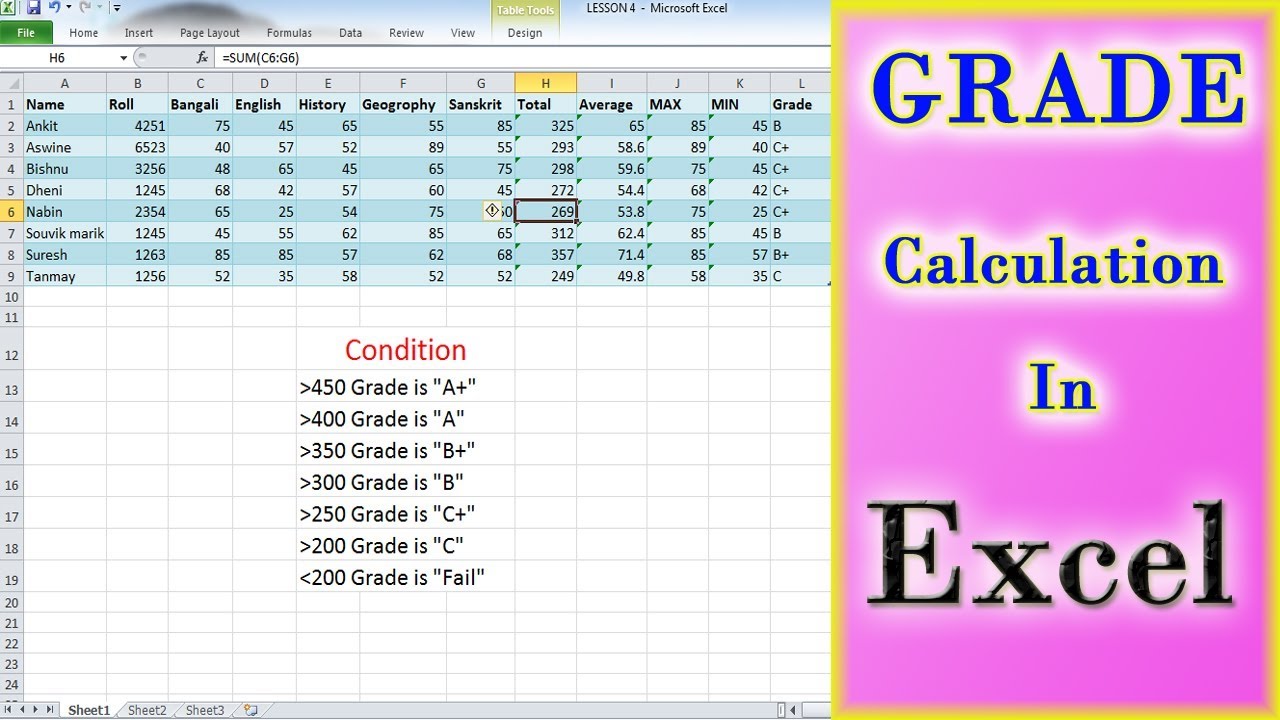
The Formula for Grade in Excel
To use the formula for the grade in Excel, a combination of logical functions (IF, Nested IF, AND, OR) and operators such as “>=, <=, >, <, =” must be employed. According to the grading system, these functions and operators help assign a proper grade.
