Calculating the correlation coefficient between two data sets is a common task in statistics and data analysis. The correlation coefficient provides a measure of the strength and direction of the linear relationship between two continuous variables. In Excel calculating the correlation coefficient is easy using the built-in CORREL function.
In this step-by-step guide, you’ll learn how to calculate the correlation coefficient in Excel using real-world examples.
What is Correlation Coefficient?
The correlation coefficient, usually denoted by r, measures the strength and direction of the linear relationship between two continuous variables It is a statistical measure that ranges from -1 to 1
-
A correlation coefficient of -1 indicates a perfect negative linear relationship between the variables. As one variable increases, the other decreases.
-
A correlation coefficient of 0 indicates no linear relationship between the variables. The variables are completely independent of one another.
-
A correlation coefficient of 1 indicates a perfect positive linear relationship. As one variable increases, the other variable also increases.
The closer the correlation coefficient is to -1 or 1, the stronger the linear relationship between the variables. The closer it is to 0, the weaker the linear relationship.
The sign of the correlation coefficient indicates the direction of the relationship. A positive value indicates a positive relationship, while a negative value indicates a negative or inverse relationship.
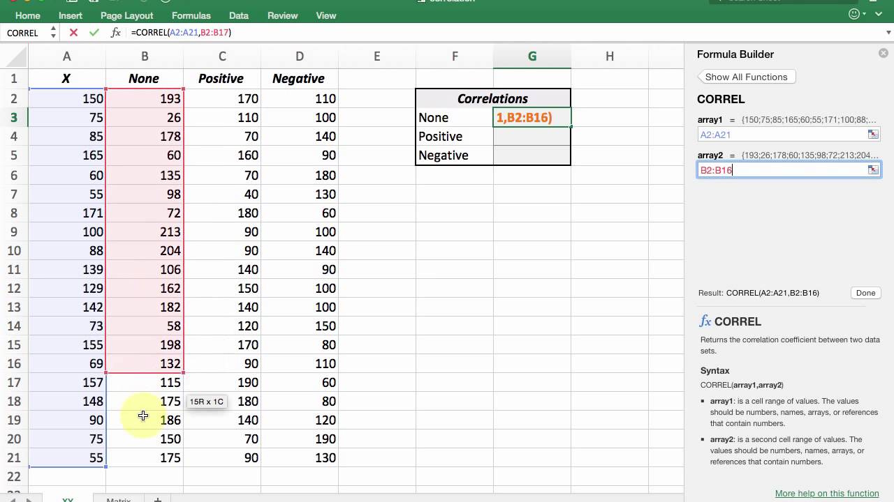
Using Excel’s CORREL Function
Excel provides the CORREL function to calculate the correlation coefficient between two data sets. The syntax of the CORREL function is:
=CORREL(array1, array2)
Where:
- array1 is the first data set
- array2 is the second data set
To use CORREL, simply provide the two arrays of data as the function arguments. Here are some important things to keep in mind:
- The arrays must have the same number of data points.
- The data must be continuous variables.
- Blank cells, text, and logical values are ignored.
- The arrays can be a cell range or array constants.
Let’s look at an example to see how to use CORREL in practice.
Example of Calculating Correlation Coefficient in Excel
Let’s say we have the following two data sets representing the study time and test scores of 7 students:
| Study Time (hours) | Test Score (%) |
|---|---|
| 2.5 | 85 |
| 3 | 90 |
| 4 | 92 |
| 2 | 80 |
| 5 | 95 |
| 1 | 75 |
| 3 | 88 |
To find the correlation coefficient between these two data sets using Excel’s CORREL function:
-
Select a blank cell, let’s say D1, where you want to output the correlation coefficient.
-
Type the formula
=CORREL(A2:A8,B2:B8)and press Enter.
This uses the CORREL function with the two data ranges as the arguments to calculate the correlation coefficient.
- The result 0.6628 is the correlation coefficient between study time and test scores for the given data.
The positive value indicates a positive relationship – as study time increases, test scores also tend to increase. The coefficient is moderately strong at 0.6628, indicating a reasonably strong positive linear relationship between the variables.
Interpreting the Correlation Coefficient
When interpreting a correlation coefficient, consider these guidelines:
- +/- 0.1 to 0.3 = weak correlation
- +/- 0.3 to 0.5 = moderate correlation
- +/- 0.5 to 1.0 = strong correlation
A correlation coefficient of 0.6628 indicates a moderately strong positive linear relationship. While not a perfect correlation, study time and test scores clearly have an association in the expected direction.
However, correlation does not imply causation – we cannot conclude that more study time causes higher scores based solely on this correlation coefficient. Other experimental methods are needed to establish causality. The correlation coefficient is limited to measuring the strength of the linear relationship.
Correlation Matrix for Multiple Variables
You can extend this correlation analysis to more than two variables by creating a correlation matrix.
For example, say you have four variables – study time, attendance, sleep, and test score. You can calculate the correlation coefficients between each pair of variables:
| Study Time | Attendance | Sleep | Test Score | |
|---|---|---|---|---|
| Study Time | 1 | |||
| Attendance | 0.21 | 1 | ||
| Sleep | -0.31 | -0.02 | 1 | |
| Test Score | 0.67 | 0.11 | -0.41 | 1 |
To generate this matrix in Excel:
-
Enter each variable data set in columns on a worksheet
-
Use the CORREL function to calculate r between study time and each other variable
-
Repeat for each pair of variables
-
Output the results in a table as shown above
This allows you to analyze the correlation between every combination of variables, not just pairs.
Examples of Using Correlation Coefficient
Here are some examples of using the correlation coefficient in real-world data analysis:
- Determine the strength of relationship between education level and income
- Assess the linear association between age and blood pressure
- Evaluate the correlation between smoking and lung capacity
- Identify predictors of employee job performance using correlations
- Establish linear relationships in scientific experiments
- Verify linear dependencies between financial indicators
- Estimate correlations between economic factors like supply, demand, and price
The correlation coefficient has wide applications in business analytics, science, economics, social science research, and more. Excel’s CORREL function makes it easy to calculate for sample data sets.
Step-by-Step Instructions
To summarize, here are the key steps to calculate the correlation coefficient between two data sets in Excel:
-
Enter two data sets to correlate in adjacent columns on a worksheet. The data sets must have the same number of data points.
-
Select a new cell where you want to output the correlation coefficient.
-
Type the formula
=CORREL(range1, range2)using the data ranges for the two data sets. -
Press Enter to calculate the correlation coefficient.
-
The result will be a value between -1 and 1 indicating the strength and direction of the linear relationship.
-
Use the correlation matrix approach to calculate r between multiple data sets.
-
Interpret the correlation coefficient based on the guidelines for weak, moderate and strong correlations.
And that’s it! The CORREL function provides an easy way to find the linear correlation between two variables in Excel. This is a useful statistic for understanding relationships and dependencies in all kinds of data analytics and research.
Common Errors and Troubleshooting
When using CORREL, some common errors and issues may arise:
-
#NUM! error – This usually occurs if the arrays have a different number of data points. Ensure both arrays cover the same size range.
-
#VALUE! error – This happens if the arrays contain non-numeric values like text. The data must be numeric to find the correlation.
-
#DIV/0! error – If an array is constant or contains all zeroes, it will produce this error. Need variation in both data sets.
-
No correlation even if related – A zero correlation can occur for non-linear relationships. CORREL only measures linear correlation. Use other methods to check for non-linear associations.
-
Weak correlation for strong relationship – Outliers can reduce the correlation coefficient. May need to remove outliers first for an accurate measure of association strength.
Pay attention to these potential errors and limitations when using Excel’s CORREL function for correlation analysis. Double check the data inputs and linearity assumptions to obtain valid results.
The correlation coefficient is an important statistical measure to quantify the strength and direction of the linear relationship between two continuous variables. Excel’s in-built CORREL function provides a simple way to calculate it from sample data sets.
By following the step-by-step instructions, you can find the correlation coefficient between two variables. Extend this to a correlation matrix approach to analyze relationships between multiple data sets.
The correlation coefficient has many applications across business, science, social science and economics. It provides valuable insights into linear dependencies and associations. Excel empowers data analysts to easily incorporate correlation analysis into data workflows.
However, remember that correlation does not imply causation. Additional statistical techniques would be needed to establish cause-and-effect relationships. Use the correlation coefficient as a starting point for deeper data analysis to uncover meaningful patterns and predictive models.
Calculating Correlation Coefficient Excel
How to calculate correlation coefficient in Excel?
A correlation coefficient closer to +1 or -1 indicates a stronger relationship between the variables, while a coefficient closer to 0 indicates a weaker relationship. You can use Excel’s built-in CORREL function to compute the correlation coefficient between two data series. The syntax of the function is:
How do I perform a correlation analysis in Excel?
You can use the steps below to accomplish the task: Click the Data tab and the Data Analysis option on the Analysis group. On the Data Analysis dialog box that appears, select Correlation on the Analysis Tools list box and click OK.
How to calculate correlation coefficient between two data series in Excel?
You can use Excel’s built-in CORREL function to compute the correlation coefficient between two data series. The syntax of the function is: The function requires Array1 and Array2 parameters, which can be cell ranges or data series.
What is a correlation coefficient?
A correlation coefficient is a value that tells you how closely two data series are related. A commonly used example is the weight and height of 10 people in a group. If we calculate the correlation coefficient for the height and weight data for these people, we will get a value between -1 and 1.
