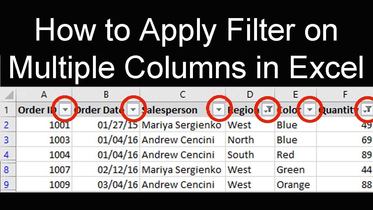
Filtering data is one of the most common and useful tasks in Excel. With a few clicks, you can show only the rows or columns that meet your specified criteria. This lets you focus on the most relevant data and hide the rest.
But what if you want to filter your data by multiple criteria? For example, you may want to show only rows where Region is ‘West’ and Sales are greater than $50,000. Excel’s standard filtering only lets you filter by one column at a time.
Luckily, there are a couple easy ways to apply multiple filters in Excel. In this article, we’ll explore two methods:
- Using manual filters on multiple columns
- Using advanced filters with complex criteria
Either way you’ll learn how to filter your Excel data by multiple conditions. Let’s get started!
Method 1: Apply Manual Filters on Multiple Columns
The easiest way to apply multiple filters is by using Excel’s manual filtering on each relevant column. Here are the steps:
Step 1: Create a Header Row
Make sure your data has a header row. This top row should contain the column labels, such as Region, Sales Rep, Sales Amount, etc. Header labels are required for filtering to work correctly.
Step 2: Select the Filter Tool
Click on the Data tab in the Excel ribbon. In the Sort & Filter group click the Filter button. This will enable filtering on your data range.
Step 3: Click the Filter Icon in Each Column Header
Look for the filter icon (it looks like a funnel) that appears in each column header. Click the icon to access the filter menu for that column.
Step 4: Select Filter Criteria
The filter menu shows all the unique values in that column. Check the boxes next to the values you want to show. For example, check ‘West’ and ‘South’ in the Region column.
Step 5: Repeat Steps for All Relevant Columns
Go through steps 3-4 for each column you want to filter by. For example, in the Sales Amount column, you may check the box for ‘>$50,000’.
This filters the table to only show rows meeting all criteria: Region is West or South, and Sales Amount is greater than $50,000.
The manual method works great for simple multiple filters. But for more complex logic, you’ll want to use…
Method 2: Advanced Filters with Complex Criteria
Excel’s Advanced Filter lets you enter complex criteria using formulas and operators like AND, OR, NOT, etc. Here’s how to use it for multiple filters:
Step 1: Set Up Your Criteria Range
On a new sheet, create a criteria range structured like this:
| Column Header | Criteria |
|

Excel assessment: Applying multiple filters on an a single sheet
How do I use a filter in Excel?
Select a cell in your data set, go to the Data tab, and pick “Advanced” to open the filter tool. Complete the same details as before, but this time, expand the criteria range to include the additional condition. Click “OK” to apply the filter. You should then see both results from the filter in the location you chose.
Can I filter multiple columns in Excel?
Yes that, right. When you apply a filter to a continuous data range, Excel allows you to filter multiple columns. In the above data, we must filter the “type” and “contributed_by” columns. This is easy if the data has multiple columns and you want to filter more than one column (two, three, or more).
How to filter multiple criteria in Excel?
Let’s follow the instructions below to filter multiple criteria in Excel! Steps: First of all, select cell G5, and write down the FILTER function in that cell. The function will be: Hence, simply press Enter on your keyboard. As a result, you will get the years when Italy was the host or champion or both which is the return of the FILTER function.
How to filter a range of data in Excel?
Select the range of data you want to filter: First, select the range or the table where you have the data on which you want to filter multiple columns. You can also click on the header of the first column, holdd the Shift key, and then click on the header of the last column to select the entire range of columns.