In this tutorial, you will find everything you need to know about sparkline charts: how to add sparklines in Excel, modify them as desired, and delete when no longer needed.
Looking for a way to visualize a large volume of data in a little space? Sparklines are a quick and elegant solution. These micro-charts are specially designed to show data trends inside a single cell.
Sparklines are a great way to visualize trends and patterns in Excel data. These mini charts fit in a single cell, condensing graphs down to their core functionality.
If you work with lots of data in Excel, sparklines can save space while still providing graphical context alongside your raw numbers.
In this guide, I’ll walk through the easy process for inserting different types of sparklines into Excel worksheets I’ll also share tips for customizing, updating, and getting the most out of these compact data visuals
What Are Sparklines in Excel?
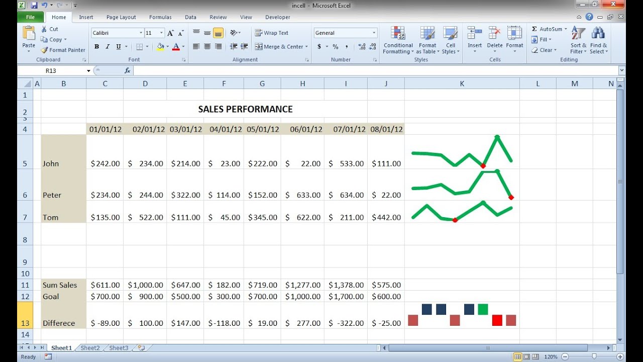
A sparkline is a tiny chart that fits in a single cell, typically in a column or row next to your data set. Sparklines condense the key information of a full size line, column, or win/loss chart down to a compact graph without axes or labels.
This minimalist graphical representation saves space while still providing visual context for the numbers in your spreadsheet. Different types of sparklines include
-
Line – Shows a trend or flow over time.
-
Column – Compares values across categories.
-
Win/loss – Displays highs, lows, and averages in columns.
Sparklines make it easy to visualize patterns, correlations, and trends across rows or columns of data. They add graphical context without taking up much room.
How to Insert Sparklines in Excel
Adding sparklines to an Excel sheet is quick and easy with the built-in Sparkline tool.
Follow these steps to insert your first sparkline:
-
Select an empty cell where you want the sparkline to appear. This should be next to the row or column of data you want to chart.
-
On the Insert tab, click the Sparklines button and hover over the type you want – Line, Column, or Win/Loss.
-
In the Create Sparklines menu, select the cells containing the data you want to chart.
-
Click OK to insert the sparkline into the selected cell.
The sparkline immediately appears in the cell, condensing your data into a compact chart.
To add more sparklines, simply drag the fill handle of the sparkline cell down to create a sparkline for each row or column in your data set. The cell references will update automatically.
Customizing Sparkline Appearance
To make your sparklines stand out, you can customize their style, color, and other formatting.
On the Sparkline Tools Design tab, you’ll find options to:
- Change the line/column color and weight.
- Switch to a different chart style or color palette.
- Show data points and customize their appearance.
- Adjust the axis min/max values.
- Hide or unhide the sparkline alongside data.
Take some time to explore all the customization and configuration options available. Formatting sparklines helps them better match your spreadsheet design.
Sparkline Limitations and Workarounds
Sparklines have some inherent limitations given their compact single cell size:
- No labels or axes to provide context.
- Hard to precisely read values from the graph.
- Limited formatting and style options.
There are some workarounds though if you need more data visualization capability:
- Add descriptive labels for rows/columns.
- Display key summary stats beside sparklines.
- Link cells to show precise data points.
- Use IKEA effect to enlarge sparkline for closer inspection.
- Switch to a full size chart for some visuals.
Sparklines are intended to provide quick, at-a-glance context. But you can supplement with other data visualization options in Excel when needed.
Tips for Effective Use of Sparklines
Here are some tips and best practices for working with sparklines in Excel:
- Place sparklines next to the source data they visualize.
- Be consistent with cell size to align sparklines in rows/columns.
- Use color to distinguish different kinds of sparklines.
- Add data point markers to draw attention to key spots.
- Show negative values in a lighter color for quick assessment.
- Link axis cells to dynamically adjust axis min/max.
- Remove gridlines and border for cleaner look when printing.
- Resize rows and columns to make sparklines stand out.
- Put sparklines on their own sheet for easy sorting and filtering.
Taking full advantage of sparkline features and functionality will help you get the most out of these compact charts.
Updating Sparklines When Data Changes
One of the benefits of sparklines is that they dynamically update when you change the underlying data they are based on. You don’t have to manually edit each time.
For example, if you add new data to a spreadsheet, just drag the sparkline cell handle down to add another sparkline plotting the new numbers.
However, if you modify existing data points, you do need to refresh the sparklines to reflect the changes. Here’s how:
-
Select all the sparkline cells you want to update.
-
Go to the Sparkline Tools Design tab.
-
Click the Refresh Data button to instantly update the selected sparklines.
Refreshing updates the cell references and displays the sparklines based on modified data.
Using Sparklines with Pivot Table Data
Sparklines are a great match for visualizing pivot table data. Just insert them beside your pivot table and refresh whenever the pivot changes.
Some good ways to incorporate sparklines with pivot tables:
- Plot totals by year, quarter, month, etc.
- Visualize trends in sum, average, or other summary values.
- Compare contributions across pivot categories.
- Show top/bottom pivot results over time.
- Link axis values to pivot filters for dynamic scaling.
Similar to adding sparklines to a standard data set, ensure your pivot table and sparkline cell widths match for proper alignment.
Sparklines provide a simple yet powerful way to add graphical context to spreadsheet data. Their compact inline design makes them a smart choice for condensing trends and patterns down to tiny cell spaces.
Now that you know how to insert, customize, and update sparklines in Excel, you can start reaping their benefits in your own workbooks. Just remember to place them carefully next to the source data for maximum impact.
With creative use of labeling, formatting, and synergies with pivot tables, sparklines enable you to get the most out of these petite yet mighty data visualization tools. They deliver an effective summary of key data insights without taking up much real estate in your spreadsheet.
Give sparklines a try today to enhance your Excel data analysis capabilities and make your worksheets more engaging and informative at a glance. The tiny charts pack a surprisingly big visual punch!
How to add sparklines to multiple cells
From the previous example, you already know one way to insert sparklines in multiple cells â add it to the first cell and copy down. Alternatively, you can create sparklines for all cells in one go. The steps are exactly the same as described above except that you select the entire range instead of a single cell.
Here are the detailed instructions to insert sparklines in multiple cells:
- Select all the cells where you want to insert mini-charts.
- Go to the Insert tab and pick the desired sparkline type.
- In the Create Sparklines dialog box, select all the source cells for Data Range.
- Make sure Excel displays the correct Location Range where your sparkline are to appear.
- Click OK.
Microsoft Excel provides three types of sparklines: Line, Column, and Win/Loss.
How to group and upgroup sparklines
When you insert multiple sparklines in Excel, grouping them gives you a big advantage â you can edit the whole group at once.
To group sparklines, this is what you need to do:
- Select two or more mini charts.
- On the Sparkline tab, click the Group button.
Done! 
To ungroup sparklines, select them and click the Ungroup button.
Tips and notes:
- When you insert sparklines in multiple cells, Excel groups them automatically.
- Selecting any single sparkline in a group selects the entire group.
- Grouped sparklines are of the same type. If you group different types, say Line and Column, they all will be made the same type.
How to Create Sparklines in Excel 2013 For Dummies
How to insert sparklines in multiple cells in Excel?
Here are the detailed instructions to insert sparklines in multiple cells: Select all the cells where you want to insert mini-charts. Go to the Insert tab and pick the desired sparkline type. In the Create Sparklines dialog box, select all the source cells for Data Range.
How to create a sparkline chart in Excel?
1. Select the cells you want represented in your sparkline chart. In this example, I’ve selected all the cells between B2 and I2. 2. In the header toolbar, select Insert, then Sparklines. 3. You should then see a dropdown menu where you can select the type of sparkline chart you want: line, column, or win-loss. I selected a line for this example.
How do I Change A sparkline in Excel?
To change between chart types, simply select the sparkline, and choose another option from Line, Column or Win/Loss. Excel will only allow a sparkline to be first created in a single cell — if a range of cells is entered into the ‘ Location Range ‘ field in the ‘ Create Sparklines ‘ dialog, an error message will be triggered.
How do I Create A sparkline?
A sparkline has the greatest effect when it’s positioned near the data that it represents. To create sparklines, you must select the data range that you want to analyze, and then select where you want to put the sparklines. The data range for the sparklines The location for the sparklines
