The tutorial shows how to make and use error bars in Excel. You will learn how to quickly insert standard error bars, create your own ones, and even make error bars of different size that show your own calculated standard deviation for each individual data point.
Many of us are uncomfortable with uncertainty because it is often associated with lack of data, ineffective methods or wrong research approach. In truth, uncertainty is not a bad thing. In business, it prepares your company for the future. In medicine, it generates innovations and leads to technological breakthroughs. In science, uncertainty is the beginning of an investigation. And because scientists love quantifying things, they found a way to quantify uncertainty. For this, they calculate confidence intervals, or margins of error, and display them by using what is known as error bars.
Error bars are an important element in Excel charts that help visualize the variability and uncertainty in data. While Excel allows you to easily add default error bars to charts, customizing error bars for each data point requires a few extra steps.
In this comprehensive guide, I will walk you through how to add individual error bars in Excel charts using a simple example. Whether you want to show custom error values, standard deviation, or percentage – this tutorial has got you covered!
What are Error Bars in Excel Charts?
Error bars visually indicate the variability or error in data points plotted on Excel charts. They represent the confidence intervals around each data point.
For example if each data point in your Excel chart represents an average of multiple measurements, error bars would show the expected range of values around that average.
![Error bars in Excel column chart][]
By looking at the error bars, you can gauge the precision and consistency in the underlying data. Wider error bars indicate higher variability in the data.
Excel allows you to add error bars to column, bar, line, area and scatter charts. You can add error bars for:
- Standard error of each data point.
- Standard deviation around the mean.
- Custom values or cell references for asymmetric errors.
Now let me show you how to add error bars in Excel charts.
How to Add Error Bars in Excel Charts
Adding default error bars in Excel charts is very easy. Just follow these steps:
- Select the chart and go to Chart Elements (+) icon.
- Check the Error Bars option.
This will add symmetric error bars to all data points showing the standard error.![Add default error bars in Excel][]
However, to customize error bars for each data point, you need to set them up as individual error bars. Let’s see how to do that.
How to Add Individual Error Bars in Excel
To add custom error bars for each data point in an Excel chart, follow these steps:
Step 1: Open Format Error Bars Pane
- Select the chart and go to Chart Elements (+) icon.
- Click the arrow next to Error Bars and select More Options.![Open Format Error Bars pane in Excel][]
This will open the Format Error Bars pane on the right side.
Step 2: Select Custom Error Amount
In the Format Error Bars pane:
- Under Error Amount, select Custom.
- Click the Specify Value button.![Select Custom error amount in Excel][]
This will open the Custom Error Bars dialog box.
Step 3: Set Positive and Negative Error Values
In the Custom Error Bars dialog box:
- Delete any existing values for positive and negative errors.
- Click in the input box and select the cell references for positive error values.
- Repeat the same for setting cell references for negative error values.
For example:![Add individual error bars in Excel][]
That’s it! The chart will now show custom error bars for each data point.
You can also type comma-separated values directly in the input boxes instead of cell references.
Now let’s go through a few examples for adding individual error bars in Excel charts.
Examples of Individual Error Bars in Excel
Let’s see how to add percentage, standard deviation, and custom error amounts as individual error bars.
Percentage Error Bars
To show asymmetric percentage error for each data point:
- In the Format Error Bars pane, select Percentage under Error Amount.
- Specify the positive and negative percentage values in the input boxes.![Percentage error bars in Excel][]
Standard Deviation Error Bars
To display symmetric standard deviation error bars:
- In the Format Error Bars pane, select Standard Deviation under Error Amount.
- Enter the number of standard deviations in the input boxes. ![Standard deviation error bars in Excel][]
Custom Error Values
To add asymmetric custom error bars:
- In the Format Error Bars pane, select Custom under Error Amount.
- Specify the positive and negative error values through cell references or directly.![Custom error bars Excel][]
This allows you full flexibility in representing error bars in Excel charts.
Tips for Adding Individual Error Bars
Here are some useful tips for working with individual error bars in Excel:
- For horizontal error bars, create an XY Scatter or Bubble chart. Other chart types only allow vertical error bars.
- To remove error bars for a specific data point, enter zero for the error amount.
- If you get an error while adding cell references, make sure to delete any existing values first.
- You can select the error bar and hit Delete key to remove it from the chart.
- To quickly open the Format Error Bars pane, double-click on the error bar.
- Right-click on the error bar and select Format Error Bars to customize it.
- Use wider error bars styles and dark colors to attract attention to the variability.
So that’s how you can add custom error bars for individual data points in Excel charts.
Error bars are a simple yet effective way to communicate data variability in Excel charts. By following the steps in this guide, you can:
- Add default symmetric error bars showing standard error.
- Customize asymmetric error bars for each data point.
- Show percentage, standard deviation or custom error values.
Mastering small chart design elements like error bars goes a long way in improving your data visualization skills.
So try adding meaningful error bars next time you create an Excel chart. Your readers will appreciate it!
How to make error bars for a specific data series
Sometimes, adding error bars to all data series in a chart could make it look cluttered and messy. For example, in a combo chart, it often makes sense to put error bars to only one series. This can be done with the following steps:
- In your chart, select the data series to which you want to add error bars.
- Click the Chart Elements button.
- Click the arrow next to Error Bars and pick the desired type. Done!
The screenshot below shows how to do errors bars for the data series represented by a line: 
As the result, the standard error bars are inserted only for the Estimated data series that we selected: 
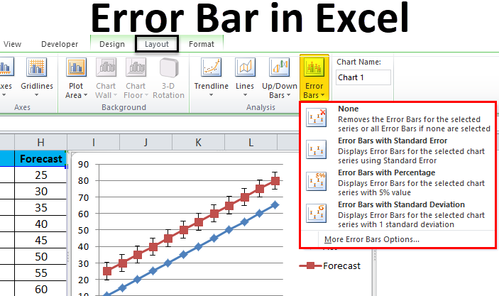
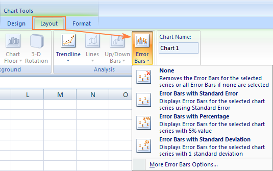
How to do error bars in Excel 2010 and 2007
In earlier versions of Excel, the path to error bars is different. To add error bars in Excel 2010 and 2007, this is what you need to do:
- Click anywhere in the chart to activate Chart Tools on the ribbon.
- On the Layout tab, in the Analysis group, click Error Bars and choose one of the following options:
How to Add Individual Error Bars in Excel
How to add Error bars in Excel?
First, select the chart in which you want to add error bars. Then, click on the Plus sign (+) next to the chart. A chart element box will appear. Make sure the tick mark is at the Error Bars box. Click on the arrow next to it. A list of items will appear that you can add to your chart. Note: You can include the error bars as follows in your chart.
How do I add a custom error bar to an Excel chart?
The custom error bar option is the method shown below. The key to adding custom error bar or confidence interval data to an Excel chart is to calculate the difference between the upper and lower error values and the series values to be plotted. Include these values in your data table to load into the chart.
Can I add Error bars to a line chart in Excel?
Yes, you can add error bars to your line chart in Excel. While creating your line chart, select the chart and click on the Chart Elements button. Then enable the Error Bars option. After that, customize the error bars as needed to make them visible on the chart.
How to calculate error bar in Excel?
Excel takes the Positive Error Value and adds it back to the series value to plot the right-hand end of the error bar. Excel takes the Negative Error Value and subtracts it from the series value to plot the left-hand end of the error bar. Add the error bar data to your data table for the chart — see calculate error bar data above for more details.
