We generally use VLookup and other lookup functions for finding the common entries from 2 lists. Here, I have given formula for finding the differences in the lists. in A column, we have recipients of the meeting invite and in B column we have the attendees list. We want to find out who were all not attended the meeting. Here I have used COUNTIF function for finding the attendees, keeping attendees list in the range and recipient list in the criteria. It returns the count as 0s and 1s; 0s for the not attended and 1s for the attendees. After that, using FILTER function, and checking if the COUNTIF function results is zero. Filter function return the not attended list.
Maybe you can use the LET function, which allows you to create a variable and use it within a formula.
Otherwise, if it has to be a formula, the example would have to be a Countif function in column C and then the filter function in column D. Something like that.
Comparing two lists in Excel is a common task analysts and data professionals need to perform regularly However, with over a million different ways to manipulate data in Excel, it can be challenging to determine the best approach
In this comprehensive guide I will share the top 10 methods for comparing two lists or datasets in Excel, with simple step-by-step instructions and examples. Whether you’re a beginner looking for a quick way to spot differences or an expert seeking a dynamic solution there’s a technique here that will meet your needs.
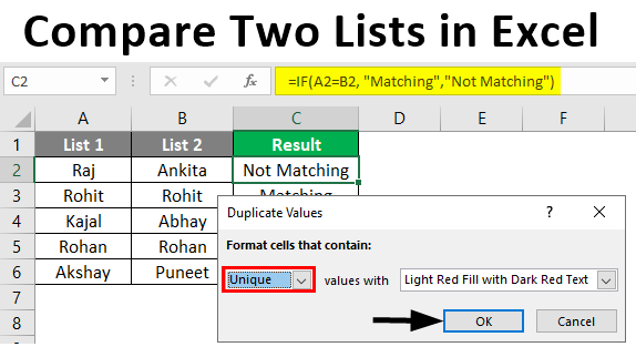
1. Use Conditional Formatting to Highlight Unique Values
The fastest way to visually compare two lists is with Excel’s Conditional Formatting tool. Here’s how:
-
Select both lists you want to compare.
-
Go to Home > Styles > Conditional Formatting > Highlight Cells Rules > Duplicate Values.
-
In the Duplicate Values dialog box, select “Unique” from the dropdown.
-
Pick a formatting style to highlight unique values.
-
Click OK.
This will automatically highlight values that only appear in one list but not the other, allowing you to quickly identify differences. The best part is it takes only seconds to set up!
2. Show Differences with Custom Conditional Formatting
You can also build custom rules with formulas to compare lists and highlight matches and discrepancies. Here are the steps:
-
Select the range to apply formatting to.
-
Go to Home > Conditional Formatting > New Rule.
-
Select “Use a formula to determine which cells to format”.
-
Enter a formula like
=COUNTIF(List2,List1)>0 -
Pick a format for matches.
-
Enter a formula like
=COUNTIF(List2,List1)=0 -
Pick a format for discrepancies.
-
Click OK.
With this flexible approach, you can define any criteria to visually flag differences between your lists.
3. Compare with the MATCH Function
The MATCH function allows you to check if an item in one list exists in another list. Here is the basic syntax:
=MATCH(lookup_value, lookup_array, 0)
This returns the position of the lookup value in the lookup array, or #N/A if no match is found.
To get a simple match output:
=IF(ISNA(MATCH(A2,List2,0)),"No Match","Match")
This displays “Match” or “No Match” based on whether List2 contains the lookup value.
4. Compare with XMATCH (Excel 365)
XMATCH is an upgraded version of MATCH introduced in Excel 365. The syntax is similar:
=XMATCH(lookup_value, lookup_array)
But it adds new search modes and doesn’t require you to specify the match type.
To return a Boolean match result:
=IF(ISNUMBER(XMATCH(A2,List2)),"Match","No Match")
XMATCH also supports spill ranges, so you can match an entire column without dragging the formula down.
5. Identify Missing Values with VLOOKUP
VLOOKUP is another common lookup function perfect for comparing lists:
=VLOOKUP(lookup_value, lookup_array, 2, FALSE)
If a match is found, it returns the corresponding value. If not, you get #N/A.
To generate a match output:
=IF(ISNA(VLOOKUP(A2,List2,2,FALSE)),"No Match","Match")
VLOOKUP also works nicely with spill ranges in Excel 365.
6. Compare with XLOOKUP (Excel 365)
XLOOKUP is the latest addition that replaces VLOOKUP with more flexibility:
=XLOOKUP(lookup_value, lookup_array, return_if_not_found)
The third argument lets you specify what to return when no match is found, instead of just #N/A.
To get a match output:
=IF(ISNUMBER(XLOOKUP(A2,List2,"No Match")),"Match",XLOOKUP(A2,List2,"No Match"))
This takes advantage of the new functionality in XLOOKUP.
7. Count Matches with COUNTIF
You can also leverage the COUNTIF function to compare lists:
=COUNTIF(lookup_range,lookup_value)
This counts the occurrences of the lookup value in the lookup range.
To generate a Boolean output:
=IF(COUNTIF(List2,A2)>0,"Match","No Match")
COUNTIF offers a simple way to check for matches without dealing with #N/A errors.
8. Combine Lists into a PivotTable
PivotTables have a built-in feature to highlight duplicates when you add both lists as sources. Here are the steps:
-
Select both lists and create a PivotTable.
-
Add field to Rows area twice to list each record separately.
-
Right click on a row item, Select Duplicate.
-
Filter to only show (Duplicate).
This neatly lists out duplicate records, allowing you to identify matches. The PivotTable approach scales well if your lists contain additional columns of data.
9. Merge Lists with Power Query
Power Query is the ideal way to compare entire tables with multiple columns. Here’s how to merge two lists:
-
Get data from each list into its own query.
-
Select one query and go to Home > Merge Queries.
-
Select the other query as the merge source.
-
Pick a join type like Left Outer to show rows in List 1 with no match in List 2.
The merged result highlights rows that only exist in one table, providing an automated way to compare lists.
10. Combine Lists into a Data Model
If your versions of Excel support Data Models, you can import both lists as tables into the Data Model. This automatically establishes relationships between matching columns.
Then, create a PivotTable from the Data Model, and add fields to the Rows area. Filter to “(Blank)” on the secondary list field to show unmatched rows.
The Data Model gives you additional flexibility to relate data from multiple sources.
Summary
In this guide, we explored 10 helpful ways to compare two lists or datasets in Excel, ranging from quick conditional formatting tricks to more advanced Power Query and Data Model techniques.
Here is a summary of the top options:
- Conditional Formatting – Quickly highlight unique or duplicate values
- Custom Rules – Flexible custom formulas to show matches and differences
- MATCH – Lookup function to find matches
- XMATCH – More powerful version of MATCH (Excel 365)
- VLOOKUP – Return matches or #N/A
- XLOOKUP – VLOOKUP replacement with more functionality
- COUNTIF – Count occurrences to identify matches
- PivotTables – Built-in duplicate identification
- Power Query – Merge and compare full tables
- Data Model – Relate data from multiple sources
No matter what kind of lists you need to compare or what version of Excel you use, this guide outlined techniques that can meet your specific needs. Try out some of these methods next time you need to spot differences between two lists!
Related Discussions View all
by indyhighlander on April 06, 2024
by marturzyca on January 24, 2024
by Mohamed_Hanno on December 31, 2023
