To multiply columns in Excel, use a formula that includes two cell references separated by the multiplication operator (asterisk). Then, use the fill handle to copy the formula to all other cells in the column. You can also use the PRODUCT function, an array formula, or the Paste Special feature.
Microsoft Excel is full of useful features, including those for performing calculations. If there comes a time when you need to multiply two columns in Excel, there are various methods for doing so. Well show you how to multiply columns right here.
Multiplying columns in Excel is a common task for many spreadsheet users. Whether you’re analyzing data creating budgets, or performing any other calculations, you’ll likely need to multiply two or more columns together at some point.
Luckily, Excel provides several easy ways to multiply entire columns in your worksheets. In this comprehensive guide, you’ll learn multiple methods to multiply columns in Excel using formulas and functions.
Why Multiply Columns in Excel?
Here are some of the most common reasons you may need to multiply columns in Excel
-
Calculate total cost or sales amounts If you have one column containing prices and another with quantities sold, you can multiply them to get the total sales or cost amounts
-
Create budgets: Multiplying hourly rates by the estimated hours gives you project budgets. Multiplying monthly recurring expenses by 12 calculates the annual costs.
-
Analyze data and metrics: Multiplying columns lets you analyze how different variables interact and impact each other. For example, you can see how price increases affect total revenue.
-
Scale values: Multiplying by a certain number lets you quickly scale up or down the values in a column. Converting measurements from inches to centimeters is a common example.
-
Model scenarios: By multiplying columns by different percentages, you can model best-case and worst-case scenarios for financial projections.
As you can see, multiplying columns has many uses in Excel. So let’s look at how to do it.
Use the Multiplication Operator
The most straightforward way to multiply columns in Excel is by using the multiplication operator (*).
Simply create a formula using cell references from the columns you want to multiply, separated by the asterisk.
For example, to multiply column A and B starting in row 2, use this formula in C2:
=A2*B2Then copy the formula down the column to multiply the remaining rows. The cell references will update automatically thanks to Excel’s relative referencing.
Tip: To multiply more than two columns, add additional cell references. For example, to multiply columns A, B and C, use:
=A2*B2*C2This method works great for multiplying a few columns. But if you need to multiply many columns, a function may be better.
Use the PRODUCT Function
Another way to multiply columns in Excel is with the PRODUCT function. The syntax is:
=PRODUCT(value1, value2, ...)Where value1, value2, etc. are the ranges or cells you want to multiply.
Simply provide the column references as the function arguments to multiply them.
For example, to multiply columns A and B, use this formula:
=PRODUCT(A:A, B:B)The PRODUCT function automatically multiplies all the values in the referenced columns and returns the result.
Tip: The PRODUCT function accepts up to 255 arguments, letting you multiply a large number of columns if needed.
The main advantage of PRODUCT is you don’t need to copy the formula down the column. You enter it once and it handles the entire column multiplication.
Use an Array Formula
For another method without copying formulas, you can use an array formula.
Array formulas let you perform calculations across entire columns in one formula, without needing to copy it down.
Here is the array formula to multiply columns A and B:
=A2:A10*B2:B10Make sure to press Ctrl + Shift + Enter after typing the formula to input it correctly as an array formula. Excel will place curly brackets {} around the formula to indicate it.
The array formula multiples all values in the referenced ranges and outputs the results in a single column.
You can include more columns simply by adding more references, like:
=A2:A10*B2:B10*C2:C10Array formulas require a couple more keystrokes but let you skip copying formulas down columns.
Use the Paste Special Option
Here is one more creative way to multiply columns using Excel’s Paste Special feature. The steps are:
-
Copy one of the columns you want to multiply and paste it in the output column.
-
Copy the other column.
-
Right-click the output column and select Paste Special.
-
Choose Multiply as the operation.
For example, to multiply columns A and B into column C:
-
Copy column B and paste into C.
-
Copy column A.
-
Right-click column C and pick Paste Special > Multiply.
This multiplies the copied column A by the existing values in column C.
While this approach takes a few more clicks, some users may find it easier than remembering formulas.
When to Use Absolute vs Relative References
One key decision when multiplying columns in Excel is whether to use relative or absolute cell references in your formula.
Relative references (A1, B2, etc.) will automatically change when copying the formula to other cells. This is normally what you want.
Absolute references ($A$1, $B$2, etc.) remain fixed when copying formulas. You’d use these if you always want to multiply by the same column.
Deciding when to use relative vs. absolute references takes some practice in Excel. Some examples:
-
If multiplying by a tax rate column, use an absolute reference so it stays fixed when copying.
-
When multiplying two data columns, use relative references so they change down the rows.
-
To multiply by a conversion factor like inches to cm, use an absolute reference to keep it constant.
In practice, Excel’s relative cell referencing often takes care of this for you. But it’s good to understand absolute references for special cases.
Errors to Avoid When Multiplying Columns
While multiplying columns in Excel is straightforward, a few errors can trip you up:
-
Formulas not copying – Remember to press Enter after typing the formula, then double-click the fill handle to copy down.
-
#VALUE errors – This occurs if entire columns don’t contain numbers. Reference specific ranges containing data.
-
#REF errors – Check for deleted rows or columns. Edit the formula range as needed.
-
Wrong calculation results – Double check if you used the correct relative and/or absolute references.
-
Copying column width – When copying a column, be sure to uncheck this option in the Paste Special box.
With a little practice, you’ll be multiplying columns in Excel flawlessly.
Next Steps
Multiplying entire columns is a critical Excel skill all users should know. The key options include:
- Multiplication operator
- PRODUCT function
- Array formulas
- Paste Special
Test the different methods and find one that suits your style. With the right technique, you can breeze through column multiplications in Excel.
For more examples, check out the advanced tutorial on multiplying columns in Excel. Up next, learn how to divide columns in Excel using similar methods. The possibilities are endless when you master these core skills!
Use the Multiplication Operator
Just like multiplying a single set of numbers with the multiplication operator (asterisk), you can do the same for values in columns using the cell references. Then, use the fill handle to copy the formula to the rest of the column.
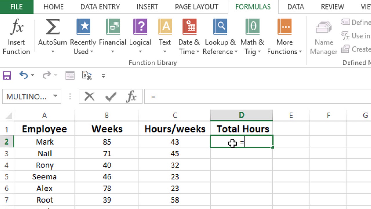
Select the cell at the top of the output range, which is the area where you want the results. Then, enter the multiplication formula using the cell references and asterisk. For example, well multiply two columns starting with cells B2 and C2 and this formula:
When you press Enter, youll see the result from your multiplication formula.

You can then copy the formula to the remaining cells in the column. Select the cell containing the formula and double-click the fill handle (green square) in the bottom right corner.

The empty cells below fill with the formula and the cell references adjust automatically. You can also drag the handle down to fill the remaining cells instead of double-clicking it.

If you use absolute cell references instead of relative ones, they will not automatically update when you copy and paste the formula.
Pull in the PRODUCT Function
Another good way to multiply columns in Excel is using the PRODUCT function. This function works just like the multiplication operator. Its most beneficial when you need to multiply many values, but it works just fine in Excel to multiply columns.
The syntax for the function is PRODUCT(value1, value2,...) where you can use cell references or numbers for the arguments. For multiplying columns, youll use the former.
Using the same example above, you start by entering the formula and then copy it down to the remaining cells. So, to multiply the values in cells B2 and C2, youd use this formula:

Once you receive your result, double-click the fill handle or drag it down to fill the rest of the column with your formula. Again, youll see the relative cell references adjust automatically.

How to Multiply Columns in Excel
FAQ
How to auto multiply in Excel?
How do I multiply columns in Excel and sum?
How do I multiply two columns in Excel?
To multiply two columns in Excel, write the multiplication formula for the topmost cell, for example: After you’ve put the formula in the first cell (C2 in this example), double-click the small green square in the lower-right corner of the cell to copy the formula down the column, up to the last cell with data:
How to multiply in Excel?
To start off, it is vital to know that formulas for multiplication in Excel begin with an equal sign (=). This indicates that Excel needs to calculate the formula. Then, you must figure out the two or more columns or cells you want to multiply. To do this, use cell references – like A1 or C3 – to specify particular cells.
What is the fastest way to multiply in Excel?
As it happens, the fastest way to do multiplication in Excel is by using the multiply symbol (*), and this task is no exception. Here’s what you do: Enter the number to multiply by in some cell, say in B1. In this example, we are going to multiply a column of numbers by percentage.
How to multiply a column of numbers by one number?
The trick to multiplying a column of numbers by one number is adding $ symbols to that number’s cell address in the formula before copying the formula. In our example table below, we want to multiply all the numbers in column A by the number 3 in cell C2. The formula =A2*C2 will get the correct result (4500) in cell B2.
