Creating a bar graph in Google Sheets is an effective way to visually compare data across categories or groups. Whether it’s sales data, revenue growth, or customer demographics, bar graphs made in Google Sheets are customizable and visually appealing.
This guide will take you through the process of creating a bar graph, from data selection to chart customization.
Bar graphs are a versatile and effective way of visually representing data. They employ rectangular bars of varying lengths or heights to display information, with each bar representing a specific category or group. The length or height of these bars signifies the values or frequencies of the data points being presented.
One of the primary advantages of using bar graphs is their ability to reveal patterns, trends, and comparisons among the data. Comparing different categories becomes much more straightforward since the bars allow for a side-by-side representation, making data interpretation more accessible and faster for the reader.
There are several types of bar graphs, such as horizontal and vertical graphs, each with its unique applications:
Bar graphs are one of the most useful and common chart types used in Google Sheets. With just a few clicks, you can turn raw data into clear and engaging visualizations
As a spreadsheet expert, I often get asked “How do I make a bar graph in Google Sheets?”. Well, you’ve come to the right place! In this comprehensive guide, I’ll walk you through the entire process step-by-step.
Why Use Bar Graphs?
Before we dive in, let’s quickly go over why bar charts are so popular:
-
Comparing Data – Bar graphs allow you to easily compare values across different categories or time periods Perfect for spotting trends and patterns
-
Visual Impact – Bars jumping off the page naturally draw the eye. Bar charts turn dry numbers into something visually striking.
-
Intuitive Design – The concept is simple – longer bars represent larger values. This makes bar graphs universally understood by all audiences.
-
Small or Large Datasets – Bar charts work great for tiny datasets with just a few data points or massive ones with hundreds of rows. Flexibility is baked in.
How to Make a Basic Bar Graph in Google Sheets
Creating a bar chart from your data range takes just a few clicks:
-
Select Data Range – Highlight the cells containing the data you want to chart. Include any row/column labels.
-
Insert Chart – Click the Insert tab and select the Chart option. A basic chart will pop up.
-
Choose Bar Chart Type – In the Chart editor panel, select “Bar chart” as the Chart type.
That’s it! Google Sheets will automatically generate a bar graph from your data. Let’s look at an example:
![Basic bar graph example][]
Now that wasn’t so hard, was it? With three quick steps, your spreadsheet data is transformed into a sleek bar chart.
But we can make things even better…
Customizing and Enhancing Your Bar Graph
The key benefit of Google Sheets is flexibility. You can customize the auto-generated chart to match your specific needs.
Here are some of the most common bar graph modifications:
- Change title – Double click the Chart title textbox to edit it
- Add axis titles – Descriptive titles help viewers understand the data
- Adjust legend – Tweak the legend position, labels, or remove it entirely
- Edit color scheme – Use colors that fit your brand or message
- Format data labels – Display value percentages, currency symbols, or custom text
- Resize bars – Make certain bars wider to emphasize importance
- Sort order – Zoom bars from smallest to largest (or vice versa)
The options are nearly endless. You have 100% creative control to build the perfect visualization.
Let’s look at an example customized bar chart: ![Customized bar graph example][]
With a few tweaks, we’ve transformed the basic chart into something that better fits the data. This entire process takes just minutes in Google Sheets.
Bar Graph Variations
Up until now, we’ve focused on standard vertical bar charts. But there are a few variations that each serve specific purposes:
- Horizontal bar chart – Flip the axis for different visual impact
- Stacked bar chart – Display subcategories within bars
- Grouped bar chart – Clustered columns for grouping related data
- 100% stacked bars – Bars always total 100% for comparisons
Don’t be afraid to experiment with different layouts. The right structure can turn a confusing chart into meaningful data storytelling.
Here is an example of a stacked 100% bar chart:![Stacked 100% bar graph example][]
Adding Sparklines to Bar Charts
Sparklines are mini charts that fit within a single cell. They work great combined with bar graphs.
For example, you could place a tiny line graph sparkline next to each bar to display year-over-year trends. This adds secondary context without cluttering up the main chart.
Here’s an example bar chart enhanced with sparkline mini charts:![Bar chart with sparklines example][]
The sparklines quickly show if the metric for that bar is trending up or down over time. A simple way to incorporate additional data.
Converting Existing Charts to Bar Graphs
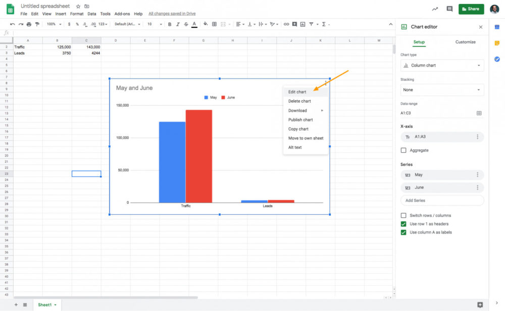
Oops! You created the wrong chart type and want to switch to a bar graph instead. No worries, it takes seconds to convert an existing chart:
-
Click on the chart to open the editor panel
-
Select the “Setup” tab
-
Change the Chart type dropdown to “Bar chart”
And that’s it! The chart will transform into a bar graph before your eyes. Much easier than deleting and starting over.
Formatting Specific Data Points
Highlighting individual data points is a great way to draw attention to outliers or points of interest.
Let’s say you wanted to call out a single high performing product. Here are the steps:
-
In the Chart editor, go to Customize > Series
-
Next to “Format data point”, click Add
-
Choose which data point to format
-
Select a contrasting color like red or orange
The chosen bar will now stand out from the others. Use this to direct viewers straight to the most important bits.
Adding Error Bars
Error bars visually represent uncertainty around a data point. They show a potential range for the “true” value.
Adding error bars is easy:
-
In the Chart editor, go to Customize > Series
-
Check the box for “Error bars”
-
Select the error type (fixed value or % of y-value work best)
-
Enter the error amount
Error bars are useful for scientific data or poll/survey visualizations. Just be careful not to clutter up the chart.
Bar Graphs as Templates
Creating charts and graphs from scratch every time is inefficient. The good news is that Google Sheets allows you to save any bar chart as a template.
Just right click on an existing bar graph and choose “Save as template.” You can then insert this pre-made bar chart into new spreadsheets.
Here are some smart ways to use bar graph templates:
- Template with your company color scheme and fonts
- Standard layout your team always uses
- Shell that contains pre-made labels and styling
Templates let you skip repetitive setup work and jump right into customizing the details.
Troubleshooting Common Bar Graph Issues
Of course, problems can pop up now and then when making bar charts. Here are some common issues and quick fixes:
Bars are missing labels – Edit your source data to add labels for each bar
Legend is cut off – Resize or reposition the chart area to fit the legend
Fonts changed – Update text font/size in the Chart editor Customize tab
Bar spacing looks weird – Adjust axis max/min values in the Setup tab
Can’t change title – Make sure the chart is selected before editing the title
Colors reset – Remake color changes in the Chart editor Customize tab
Hopefully these tips will help you diagnose and resolve any formatting problems that arise.
Key Takeaways and Next Steps
The ability to turn spreadsheet data into stunning bar graphs gives Google Sheets a huge leg up on basic office software. Transforming rows and columns into understandable charts takes just minutes.
Here are the key points we covered in this guide:
- Bar graphs are versatile and intuitive for all users
- Creating a bar chart only takes a few clicks
- Fully customize colors, labels, data points, and formatting
- Experiment with horizontal, stacked, and grouped layouts
- Use sparklines and templates to enhance your charts
- Switch chart types or troubleshoot issues with the built-in editor
Now that you’re a bar graph expert, try applying these skills to your own Google Sheet dashboards and reports. Impress your colleagues with beautiful, meaningful data visualizations that bring numbers to life.
Step 2: Select the Data You want to Graph
Once your data is in place, it’s time to select what you want to include in your graph. This selection is known as the ‘data range’.
Click and drag your mouse over the cells containing your data, including the column headings. For our sample data, you’ll select from A1 to B7.
The selection you make here depends on the data you want to visualize. In our case, we’re including both the months and their corresponding sales figures. Including the headers in your selection ensures that Google Sheets correctly labels the axes of your graph.
Step 3: Choose the Appropriate Graph Type
Now, click on the ‘Insert’ menu at the top of your screen, then choose ‘Chart’.
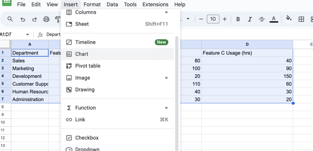
Google Sheets will automatically suggest a chart type. For sales data over time, a bar chart is typically most effective.
If the suggested chart isn’t a bar chart, or if you prefer a different style, use the Chart Editor on the right side of the screen. Here, you can change the chart type and see the effect on your data in real-time.

Supercharge your spreadsheets with GPT-powered AI tools for building formulas, charts, pivots, SQL and more. Simple prompts for automatic generation.

Making a Simple Bar Graph in Google Sheets (4/2018)
How to create a bar chart in Google Sheets?
Select the data and insert a chart into Google Sheets, similar to the picture below. You can also select the data and right-click to insert a chart. After inserting a chart in Google Sheets, you can modify the configuration to a bar chart even though Google Sheets will initially try to interpret the data and configure the chart itself.
How do I turn a chart into a bar graph?
To turn this chart into a bar graph, click on the Chart Type dropdown menu and select the Bar Chart option You can also select the Stacked Bar Chart or 100% Stacked Bar Chart options to stack all your data series into a single bar per category on the Y-Axis
How to put error bars in Google Sheets?
Here’s how to put error bars in Google Sheets in 4 steps. 1. Highlight and insert the values you’d like to visualize 2. Google Sheets automatically visualizes your data as a pie chart. To change it, click on the chart type drop-down and then select a column. Here’s what your chart should look like… 3.
