How to Unhide All Rows in Excel with 3 Simple Methods

And you don’t want to spend too much time identifying them so you can unhide them?

This guide shows you exactly how to unhide rows (and columns) in Excel in just a few minutes.

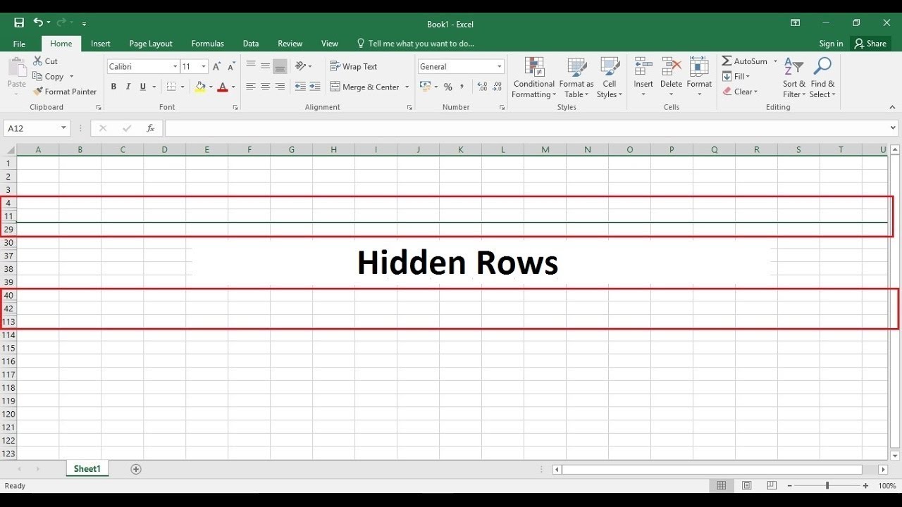
When analyzing and presenting data in Excel, you may frequently hide certain rows to simplify your spreadsheet and draw attention to the most important information.

But once your work is done, you likely want to restore the full data set with all rows visible again

Manually unhiding rows one by one would be extremely tedious. Thankfully, Excel provides quick shortcuts to unhide all rows in just a few clicks

In this guide, you’ll learn:

What happens when you hide rows in Excel
3 methods to unhide all rows at once
How to permanently delete hidden rows
Important tips for unhiding rows
Additional row visibility options in Excel

Let’s dive in to restoring hidden rows and understanding how row visibility works in Excel!

What Happens When You Hide Rows in Excel?

Before unhiding rows, let’s briefly explain what happens when you hide them in the first place:

Hiding rows simply toggles their visibility off. The data remains intact.
Hidden rows will not be displayed on your spreadsheet or printed.
Formulas automatically adjust their ranges to skip hidden rows during calculations.
Filtering will exclude hidden rows to avoid showing blank filtered results.
Charts and PivotTables don’t include hidden row source data by default.
Hidden rows maintain their styles, formatting, width settings, and more.
Other sheets in the same workbook are unaffected. Hiding only applies to the active sheet.

Now that you understand row hiding behavior, let’s undo it by unhiding rows.

Method 1: Unhide All Rows with Ctrl + Shift + 9

The fastest way to unhide all rows in Excel is using the keyboard shortcut Ctrl + Shift + 9:

Select any cell on the sheet with hidden rows.
Press Ctrl + Shift + 9 on your keyboard.
All previously hidden rows will instantly become visible again!

This shortcut unhides every hidden row on the entire sheet in one go. No need to select columns or a range first.

Just tap Ctrl + Shift + 9 whenever you want to restore all row data easily.

Method 2: Unhide All Rows from the Right-Click Menu

You can also unhide all rows through the right-click context menu:

Right-click on any cell in the sheet.
Select Unhide from the menu.
All hidden rows will immediately reappear on your spreadsheet.

The right-click menu provides quick access to unhide all if you prefer using your mouse.

Method 3: Unhide from the Excel Ribbon

The traditional way to unhide rows is via the Excel ribbon:

Click on the Home tab.
Click Format > Unhide Rows.
All hidden rows will become visible once again.

Some users may be more comfortable using the ribbon instead of shortcuts or right-click menus. All three methods produce the same instant results.

Permanently Deleting Hidden Rows

Unhiding restores rows to their previous visible state. But you can also permanently remove hidden rows from Excel if desired:

Select the entire used range of columns (Ctrl + A with first row selected).
Right click and choose Delete.
Click Shift cells up and OK.

This will delete hidden rows while shifting up remaining data to close gaps. Filter for blanks first to delete all blank hidden rows only.

Tips for Unhiding Rows in Excel

When working with hidden rows in Excel, keep these tips in mind:

Unhide regularly to avoid losing track of hidden data.
Double check there are no unintended consequences of unhiding rows.
Sort all blank hidden rows together before deleting to avoid removing data.
Add comments noting why certain rows are hidden for future reference.
Adjust column widths and formats with care if unhiding changes layout.
Unhide rows one by one if only certain rows need to reappear.
If rows suddenly disappear, press Ctrl + Shift + 9 to quickly unhide all.

Mastering row visibility will take your Excel skills to the next level!

Other Row Visibility Options in Excel

In addition to hiding and unhiding, Excel provides other helpful options to manage row visibility:

Filter to temporarily view subsets of row data.
Freeze panes to keep some rows visible as you scroll.
Split panes to see different row sections simultaneously.
Outline groups to collapse and expand grouped rows together.
Conditional formatting to highlight or gray out rows based on rules.
Sorting to move rows out of their original order.

Combine row unhiding with these other techniques for ultimate control over the rows Excel displays.

Next Steps for Unhiding Rows

Now you have 3 simple methods to instantly unhide all rows in Excel:

Ctrl + Shift + 9 – The fastest keyboard shortcut.
Right-click Unhide – Quick access from context menu.
Format > Unhide Rows – Standard approach via the ribbon.

Remember to permanently delete any hidden rows you no longer need. And leverage other visibility options like freezing panes and filters.

Mastering control of hidden rows will take your Excel expertise to the next level. Empower yourself to showcase the exact data you want with these unhiding techniques.

unhide all rows in excel

Unhide individual or multiple rows

Sometimes, you don’t want to unhide all rows, but just a specific row, or several specific rows.

To unhide multiple rows, use the same method as before:

1. Select the cell above the hidden rows, hold down your left mouse button and drag over the hidden rows – selecting them and the row below the hidden rows.

2. Right-click any of the 2 visible selected rows.

And voila! The rows are visible

Unhide first row in Excel

Unhiding the first row can be particularly tricky – if you don’t know how.

Because, how can you select it if you can’t “drag over” it, like with other hidden rows?

Luckily, there’s another way to select that first hidden row.

1. To the left of the formula bar there’s a name box. Write “A1” in it.

Now, cell A1 is selected.

2. On the right side of the Home tab, click Format.

3. Hover the cursor over ‘Hide & Unhide’ and click ‘Unhide Rows’.

Now, the first row is visible again

PRO TIP:

If you find the above method for unhiding the first row a bit too cumbersome, try this instead.

You can actually select the hidden first row by holding down the left mouse button and “dragging over” it.

You just need to start dragging from row 2 and then drag in an upwards motion that ends on row 0 (the grey triangle).

After that, just right-click row 2 and click Unhide.

Note: it’s not enough to just select row 2. You need to drag over row 1.

How to unhide all rows in Excel 2018

How to unhide all hidden rows & columns in one fell swoop?

Here’s how to unhide all the hidden rows and all the hidden columns in one fell swoop. 1. Select all the cells in the spreadsheet by clicking the ‘Select All’ button. Or you can use the Ctrl + A shortcut. 2. Right-click any of the selected rows and click Unhide. This unhides all the hidden rows. 3.

How to unhide a column in Excel?

1. Select all the cells in the spreadsheet by clicking the ‘Select All’ button. Or you can use the Ctrl + A shortcut. 2. Right-click any of the selected rows and click Unhide. This unhides all the hidden rows. 3. Right-click any of the selected columns and click Unhide. This unhides all the columns.

How do I find a hidden row in Excel?

Double-click the Excel document that you want to use to open it in Excel. Find the hidden row. Look at the row numbers on the left side of the document as you scroll down; if you see a skip in numbers (e.g., row 23 is directly above row 25 ), the row in between the numbers is hidden (in 23 and 25 example, row 24 would be hidden).

How do I unhide a range of rows in Excel?

Unhide a range of rows. If you notice that several rows are missing, you can unhide all of the rows by doing the following: Hold down Ctrl (Windows) or ⌘ Command (Mac) while clicking the row number above the hidden rows and the row number below the hidden rows. Right-click one of the selected row numbers. Click Unhide in the drop-down menu.