In Excel, there are many instances when you may need to compare two columns. It is simple when there are only a few columns and rows, but as the table expands, you need to scroll horizontally or hide columns to create a comparison.
Often, it might require you to manually compare and write down as ‘Match’ or ‘Not Match’ or highlight the matching or mismatching data in each column.
Manual comparison is painstaking and might lead to erroneous data. However, there are many methods to streamline this process.
Comparing two columns in Excel is a common task that allows you to see the differences and similarities between data sets. This can help you spot errors, find duplicates, merge lists, and more.
There are a few ways to compare columns in Excel, depending on exactly what you want to compare and what you want to do with the results. In this comprehensive guide, I’ll cover the most popular methods so you can choose the right one for your needs.
Why Compare Columns in Excel?
Here are some of the most common reasons you may need to compare two columns in Excel:
-
Find duplicates or common values By comparing two lists, you can identify values that exist in both columns This allows you to remove duplicates and consolidate data.
-
Identify differences: Comparing columns makes it easy to spot discrepancies between two data sets. For example, you may have two customer lists and want to see which names are missing from each one.
-
Update data: By comparing original data to updated data, you can identify what needs to be added, removed, or changed in your spreadsheet.
-
Merge lists: You can combine two lists into one master list by comparing them and pulling in the unique values from each one.
-
Check for errors Data entry errors often get exposed when you compare columns So comparing can help you find and correct typos or other mistakes.
-
Analyze changes over time Comparing two versions of the same data (for example – this month vs last month) can reveal trends and patterns
How to Compare Two Columns in Excel
There are a few ways to approach this task in Excel. Which method you use depends on whether you want an exact match, approximate match, or just a visual comparison.
1. Use Formulas for Exact Matches
If you need to compare two columns and identify exact matches, the best way is to use Excel formulas like VLOOKUP, INDEX/MATCH, or COUNTIF.
VLOOKUP/INDEX MATCH
These formulas allow you to check whether a value in column A exists in column B. If there is a match, it will return the value. Otherwise, you’ll get an error.
Here is the VLOOKUP syntax:
=VLOOKUP(value to lookup, range to lookup, column number in range, exact match) And this is the INDEX/MATCH syntax:
=INDEX(range to return result, MATCH(value to lookup, range to lookup, 0))So you can use these formulas to get matches between two lists or to pull corresponding data from one column into another.
COUNTIF
The COUNTIF formula counts the number of cells in a range that meet a certain condition.
You can use it to compare two columns by counting how many values from column A appear in column B. The syntax is:
=COUNTIF(range to check, criteria)So for comparing two columns, it would be:
=COUNTIF(range in column B, cell in column A to check)This will return 1 if the cell value exists in column B or 0 if it doesn’t.
2. Use Conditional Formatting to Visually Compare
Another easy way to compare two columns is by using conditional formatting.
This allows you to apply visual formats like color coding to the cells so you can see matches, differences, duplicates etc. at a glance.
Here are some conditional formatting rules you can use:
-
Highlight cells that match between two ranges: This will visually identify values that exist in both columns
-
Highlight unique values: Values that exist in only one column will get highlighted
-
Highlight duplicates: Any duplicates across the two columns or within one column will stand out
So conditional formatting gives you a visual representation of the similarities and differences between two lists.
3. Compare Side by Side
You can also manually compare two columns by placing them side by side in Excel.
This works well if your goal is just to visually scan the data and check for inconsistencies or errors.
To compare columns side by side:
-
Copy or move the two columns so they are next to each other.
-
Make sure the data is sorted in the same order in both (A to Z, Z to A etc.).
-
Scan through the rows to look for discrepancies or matches.
-
Use filters to only show duplicate or unique values.
The side by side view combined with filtering gives you a quick visual comparison.
4. Use Pivot Tables to Compare Lists
Pivot tables are a great way to summarize, analyze, explore, and compare large datasets.
You can load two column lists into a pivot table and easily see counts, differences, similarities etc. between them.
To do this:
-
Create a pivot table from one data set.
-
Add the other list to the data source as well.
-
Add one column as the Rows field and the other as Values.
-
Use filters and slicers to only show certain values.
pivot tables let you manipulate the summaries to uncover insights as you compare two lists.
Tips for Comparing Columns in Excel
Follow these tips to make your column comparisons more effective:
-
Store lists to compare in tables – This allows you to dynamically reference the data in formulas with structured references like Table1[[Column1]] instead of absolute cell references.
-
Add helper column with formulas – Rather than comparing within formulas, output the results of comparisons to a helper column. This is easier to audit and modify later.
-
Copy data to remove duplicates first – When comparing for duplicates, copy the data to a new location and remove duplicates before comparing. This avoids duplicate rules getting triggered within one list.
-
Compare based on one key column – If data has multiple columns, extract a key column with IDs or names to base the comparisons on. Comparing the entire row is inefficient.
-
Sort columns alphabetically – Sorting the lists in the same order before comparing ensures matches align properly in both columns.
-
Adjust for case sensitivity – Formulas like VLOOKUP will treat Text and text as different. Use EXACT to make it case-sensitive.
-
Add conditional formatting last – Add conditional formatting after you have completed other steps like removing duplicates. This prevents duplication rules from catching irrelevant matches.
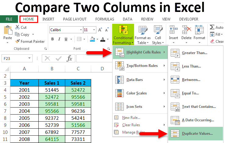
Compare Two Columns in Excel Using Conditional Formatting.
Click Home, then on Styles.
Then, follow these steps Conditional Formatting → Highlight Cell Rules → Duplicate Values.
You get a dialogue box, as shown below. From there, you must choose the values from the drop-down menu.
Apply the formatting condition on the cells. You can choose any conditions; Duplicate or Unique.
Format cells that contain: (options) values with (options).

Use Conditional Formatting to find and highlight the data that are present in both columns. Before using conditional formatting, select the columns required for comparison.
Choose Duplicate if you wish to find the names in both columns. To highlight it, choose any options: filling with colour, changing the text colour, or changing the cell border.
The last option is a Custom Format. Choose this option if you wish to highlight the cell with a colour of your choice other than the ones specified in the drop-down menu.
Another option that you can use is ‘Unique.’ Use this option if you are interested in highlighting the cells that contain data that is not repeated. That is, you wish to highlight the unique cells.
Instead of selecting Duplicate, choose Unique from the drop-down list, and apply any options, such as filling with colour, changing the text colour, or changing the cell border.
Tip: If you wish to clear the formatting you performed on the cells, click Conditional Formatting → Clear Rules → Clear Rules from Selected Cells.
You can use conditional formatting when you don’t want a third column showing the results comparing the two columns. Highlighting duplicate (matching) and unique (different) data to show which rows have the same data.
Additionally, you can use an extra column to explicitly display values indicating whether the data matches, which works for smaller tables. Alternatively, you may need to use more complex methods for large spreadsheets.
Compare Two Columns in Excel Using the EXACT() function.
If you noticed in the previous screenshot, the formula returned a Yes for matching results that had different capitalizations.
For instance, the country names had different capitalizations in rows 5, 13, and 14. The IF() returned Yes while comparing two columns containing Netherlands and netherlands, with n in lower case.
If you wish the capitalizations to be identical, use EXACT() when comparing two Excel columns and IF().
The EXACT() function compares two text strings and returns Yes only if they have the same capitalizations.
EXACT is case-sensitive but ignores formatting differences. The syntax is =EXACT(text1,text2). It takes two arguments, text1 and text2; both are required when using this function.
Let’s look at some examples. This time, EXACT() is used along with IF().
Use the formula =IF(EXACT(B4,C4), “Match”, “Mismatched”) for the IF condition to be case sensitive.
As you can observe, it returns the result as Mismatched for columns with matching results yet mismatched capitalizations.
The execution of the formula is as follows: first, the inner function is executed, and the result is returned. In the above example, the EXACT() function returns a false value to the outer function IF.
The general working of the IF condition is that if it returns true, the first argument in the function is returned. Or the second argument is returned as false.
How to Compare Two Columns in Excel to Find Differences (The Easiest Way)
How to compare two lists in Excel?
Visit our page about comparing two lists. Let’s start by comparing two columns and displaying the duplicates. 1. Display the duplicates in the first column (these values also occur in the second column). Explanation: the MATCH function in cell C1 returns the number 5 (letter A found at position 5 in the range B1:B7).
How do I compare two columns in Excel and highlight cells?
To compare two columns and Excel and highlight cells in column A that have identical entries in column B in the same row, do the following: Select the cells you want to highlight (you can select cells within one column or in several columns if you want to color entire rows).
How to compare two columns in Excel?
Another method that you can use to compare two columns can be by using the IF function. This is similar to the method above where we used the equal to (=) operator, with one added advantage. When using the IF function, you can choose the value you want to get when there are matches or differences.
How to compare two columns in Excel row-by-row?
To compare two columns in Excel row-by-row, write a usual IF formula that compares the first two cells. Enter the formula in some other column in the same row, and then copy it down to other cells by dragging the fill handle (a small square in the bottom-right corner of the selected cell). As you do this, the cursor changes to the plus sign:
