10 Easy Ways to Change Border Color in Excel Like a Pro

As an Excel power user, formatting cells and tables to make your spreadsheets visually appealing is an important skill. One simple yet effective formatting technique is changing border colors in Excel.

The default gridlines and cell borders in Excel worksheets are black. But black borders may not always complement your data or allow users to easily identify specific cells and ranges.

That’s where learning how to alter border colors comes in handy!

In this comprehensive guide, I’ll walk you through 10 quick and easy ways to modify border colors in Excel.

Whether you’re a beginner or an advanced Excel user, you’re sure to find border color-changing methods that suit your needs. Let’s get started!

Why Change Border Colors in Excel?

Before jumping into the step-by-step instructions, it’s worth understanding the key reasons for changing border colors in Excel worksheets:

• Borders in different colors help emphasize or highlight important cells, tables, and data ranges. This draws users’ attention to crucial information.

• Distinct border colors can denote different data categories like sales, expenses, inventory etc. This makes large spreadsheets more visually organized.

• Colored borders clearly distinguish specific sections or clusters of data from the rest of the sheet.

• For presentations and reports, modifying border colors improves aesthetics and makes the data easier to comprehend.

• Unique border colors can indicate cells with errors, exceptions or special formatting rules.

• When working with multiple interconnected sheets or large Excel files, consistent use of color-coded borders improves navigation.

• You can use border colors to call out cells with instructions, deadlines, notes etc.

• Finally, it simply makes your spreadsheets less monotonous and more visually engaging!

Now that you know why border colors matter, let’s get into the various methods to change them.

Use the Border Color Pencil

My favorite way to alter border colors is using the border color ‘pencil’ tool in Excel. Here are the simple steps:

• Select the Home tab and click the arrow below the Borders button in the Font group.

• Hover over ‘Line Color’ in the dropdown menu.

• Click on your desired border color from the palette.

• Your mouse pointer turns into a pencil. Click on the cell borders to color them.

• To stop coloring, hit the Esc key. This returns the pointer to normal.

The color pencil allows you to quickly change borders as needed without opening any menus. You can use it to erase borders too!

Change Border Color Using Keyboard Shortcut

If you prefer keyboard shortcuts over clicking buttons, use the handy Alt > H > B > I shortcut:

• Press Alt to open the ribbon shortcuts.

• Press H to switch to the Home tab.

• Hit B to reveal the border options.

• Finally, press I to access the color palette and select your border color.

• Your mouse morphs into a color pencil to modify borders with clicks.

• Finish up by hitting the Esc key.

This method is great when you need to repeatedly change borders across multiple cells.

Use the Format Painter

Excel’s Format Painter tool lets you copy formatting from one place to apply it elsewhere. Here’s how to use it:

• First, select the cell(s) with the border color you want to copy.

• Click the Format Painter button in the Clipboard group on the Home tab.

• Then select the cells you want to apply the border color to.

• The Format Painter automatically copies the border color over along with other formatting.

• You can keep pasting the format to multiple cell ranges until you press Esc.

Format Painter effortlessly duplicates border colors across Excel worksheets.

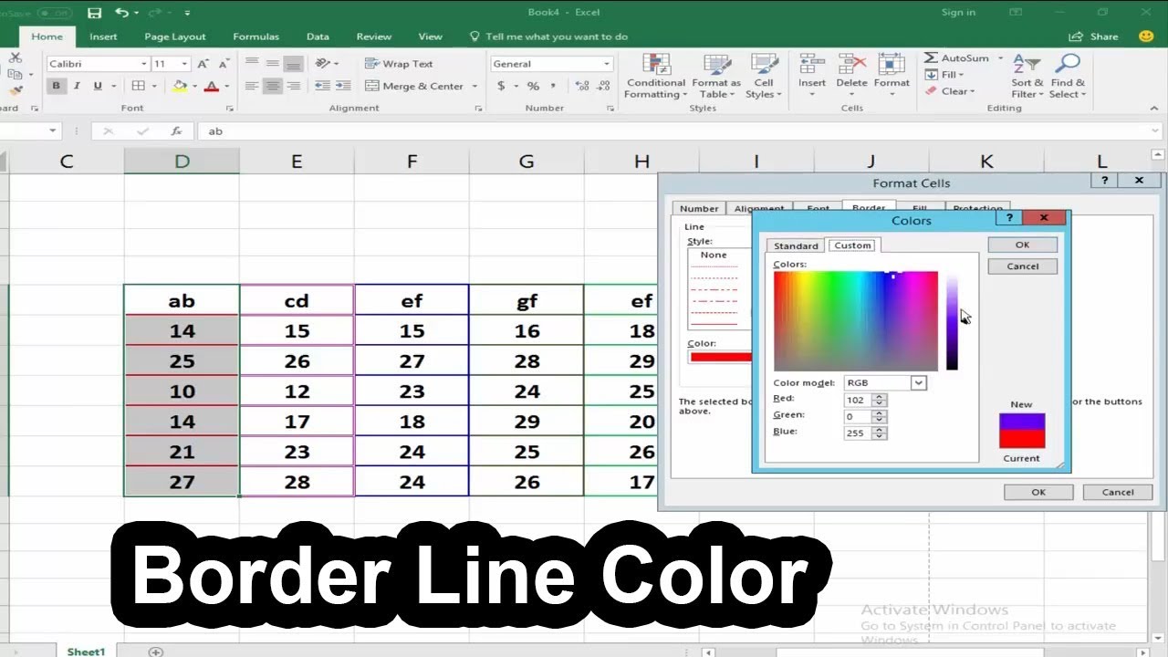
Change Borders Via the Format Cells Dialog

The Format Cells dialog box gives you precise control over formatting Excel cells. Follow these steps:

• Select the cells with borders to modify.

• Press Ctrl + 1 or right-click and choose ‘Format Cells’. This opens the Format Cells window.

• Navigate to the Border tab.

• Click the Color dropdown and pick your desired border color.

• Check the border preview box to see changes.

• Click OK to apply the color.

While this method takes a few extra clicks, it lets you tweak border styles and alignment along with color.

Use Table Styles for Quick Formatting

Custom table styles allow one-click border coloring when formatting Excel tables. Try this:

• With your table selected, open the Table Styles gallery on the Home tab.

• Click ‘New Table Style’ at the bottom.

• Name your style, select formatting preferences, and hit OK.

• Return to the Table Styles gallery and choose your custom style.

• Your table now has the customized border colors!

This technique also maintains your formatting when the table expands with new data.

Color Code with Conditional Formatting

Excel’s powerful Conditional Formatting feature can automatically color cell borders based on cell values, formulas or rules.

For example, you can highlight cells above a threshold value with a green border and those below with a red border.

Here’s how to set up such value-based color coding:

• Select the cells to format conditionally.

• On the Home tab, open the Conditional Formatting dropdown.

• Choose ‘New Rule’ and then ‘Format only cells that contain’.

• Specify the value/formula criteria and select the border color.

• Repeat to add multiple rules as needed.

You can find tons of creative ways to leverage Conditional Formatting for border colors.

Change Border Color of Chart Elements

To give your Excel charts a makeover, customize the border colors of various chart components like:

• Chart area
• Plot area
• Data series
• Titles
• Legend
• Data labels
• Axes

Simply right-click the component and choose ‘Format’. Pick border colors and lines under Fill & Line options.

This instantly modernizes dull looking charts!

Modify a Chart Data Range Border

When presenting charts built from Excel table data, use this tip to make the underlying dataset stand out:

• Click any cell inside the data table used by the chart.

• Open the Table Styles gallery on the Design tab.

• Choose a style with bold, colored borders.

The borders automatically extend to the chart’s associated data range!

Utilize Data Bars for Borders

Data bars are horizontal bars within cells representing the cell value. Enable them to essentially convert cell values into colored cell borders!

• Select the target cells and open Conditional Formatting > Data Bars.

• Pick a data bar fill color. Higher values produce wider colored bars resembling borders.

You can combine this hack with traditional border colors for a dual-border effect.

Change Default Row & Column Border Colors

Tired of constantly having to re-color black borders? Override the defaults with these steps:

• Go to File > Options > Advanced.

• Under ‘Display options for this worksheet’, pick a color for gridlines.

• Scroll down and enable the ‘Use colors from Themed Rows and Columns’ checkbox.

• Choose your preferred row and column border colors. Hit OK.

This globally alters the default border appearance in that sheet!

Use Excel Tables for Custom Borders

While Excel tables have predefined styles, you can create fully customized styles with unique border colors:

• With your data selected, click ‘Format as Table’ on the toolbar and pick custom table style.

• Give your style a name under ‘Table Element’ formatting.

• Open the Format Cells dialog to modify border color and style.

• Save your new style and format the table with it.

Let your creative juices flow with custom table border colors!

That concludes this comprehensive guide to changing border hues in Excel worksheets.

While the default black borders work fine, colored borders help organize complex datasets, highlight exceptions, and make your files visually striking.

The techniques covered above range from swift color changes using presets to fine border customizations.

Hopefully, you now have the confidence to give those boring black borders the boot and implement the border coloring method that meets your needs!

So try out a few options from this list and breathe new life into your Excel workbooks with vibrant, meaningful border colors.