How to Merge Tables in Excel: A Step-by-Step Guide

Working with multiple tables in Excel can get messy pretty quickly Luckily, Excel provides several straightforward methods for merging two or more tables into one consolidated dataset.

In this comprehensive guide, we’ll walk through the top techniques for combining Excel tables based on one or more common columns. Whether you’re looking to merge tables across worksheets or within the same sheet, these steps will show you how to get it done smoothly.

Why Merge Excel Tables?

Merging tables in Excel serves several purposes:

• Consolidates separate sets of related data into one organized table for easier analysis and visualization

• Allows you to combine Excel tables with duplicate column values by matching rows

• Lets you integrate Excel data from different worksheets or workbooks into a master table

• Helps remove data redundancy and inconsistencies across multiple tables

• Provides a clean overview of all relevant data in one place

By merging Excel tables intelligently, you can save time wrangling messy datasets and focus on deriving insights.

Prerequisites for Merging Excel Tables

Before learning how to merge tables in Excel, there are a few key prerequisites:

• The tables should contain at least one common column with duplicate values to match rows during the merge. This acts as the key for combining the datasets.

• The entries in the common columns should have the same data types and formatting in both tables.

• If possible, sort the values in the common columns alphabetically or numerically so the rows match properly during merging.

• Ensure that the tables have headers in the top row since some merge methods rely on the header names.

• The tables need to be formatted as official Excel tables using Ctrl + T or the Format as Table command.

With that background covered, let’s look at the step-by-step process for 5 of the most popular techniques to merge Excel tables.

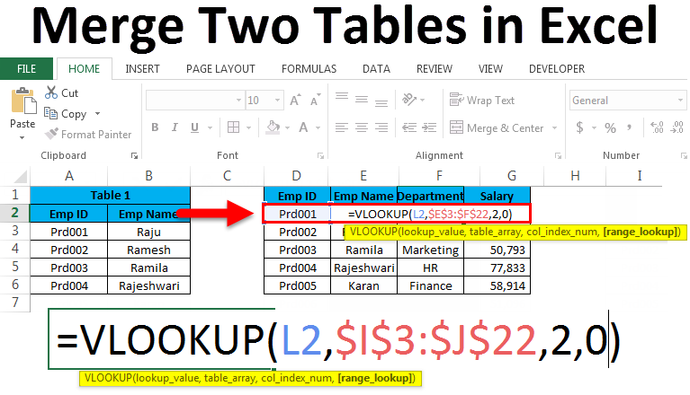
1. Merge Tables Using the VLOOKUP Function

The VLOOKUP function allows you to pull corresponding data from one Excel table into another based on a common column match.

Here are the steps to merge two tables with VLOOKUP:

1. Identify the common column between Table 1 and Table 2. This will contain the lookup values.

2. Insert new columns next to Table 1 with the headers from Table 2.

3. Apply this formula in the first new column and fill down:

   =VLOOKUP([@CommonColumn],Table2[#All],ColumnNumber,FALSE)

4. Drag the fill handle to apply that VLOOKUP formula for all rows in Table 1. This will populate the new column with values looked up from Table 2.

5. Repeat steps 3 and 4 in the second new column using the next desired column number from Table 2.

6. Apply formatting to the new columns to match Table 1 style.

The VLOOKUP merge works well when the common column has duplicate values. The [#All] reference lets you lookup within the entire table.

2. Use the XLOOKUP Function

XLOOKUP is an upgraded version of VLOOKUP suited for merging Excel tables with its added flexibility. Follow these instructions:

1. Add new columns next to Table 1 with headers from Table 2, just like in the VLOOKUP method.

2. Enter this formula in the first new column and fill down:

   =XLOOKUP([@CommonColumn],Table2[ColumnWithCommonValues],Table2[OutputColumn])

3. Drag the fill handle to apply that formula to all rows. This will populate the column with values from the output range.

4. Repeat steps 2 and 3 for the next column from Table 2.

5. Apply formatting to the new columns to match Table 1.

With XLOOKUP, you can directly reference the output range instead of column numbers.

3. Use the Power Query Merge Option

The Power Query editor lets you merge two Excel tables in just a few clicks:

1. Go to the Data tab and select the ranges for Table 1 and Table 2 using Get Data > From Table/Range.

2. Go to the Home tab in Power Query and select Merge Queries > Merge Tables.

3. In the Merge dialog, select Table 1 as the top table and Table 2 as the bottom table. Pick the join type as Left Outer.

4. Expand the Table 2 column and select the columns to keep. Remove prefixes.

5. Click Close & Load and output the merged table to your desired location.

Power Query handles all the data wrangling behind the scenes and outputs a combined table.

4. Merge with Index and Match

The INDEX and MATCH combo also allows you to merge Excel tables intelligently:

1. Add new columns next to Table 1 with headers copied from Table 2.

2. Use this formula in the first new column and fill down:

   =INDEX(Table2ColumnToReturn,MATCH([@CommonColumn],Table2[CommonColumn],0))

3. Drag the fill handle to populate the column with INDEX lookups based on MATCH row positions.

4. Repeat for the second new column using the next desired column from Table 2.

5. Apply formatting to the new columns.

INDEX pulls data into Table 1 while MATCH identifies the row positions in Table 2 dynamically.

5. Copy and Paste Columns

For a quick and simple merge, you can directly copy and paste columns from Table 2 into Table 1:

1. Confirm the common column entries match positionally in both tables.

2. Select and copy the columns to add from Table 2.

3. Select the first blank cell next to Table 1 and paste the copied columns.

4. The pasted columns will now merge into Table 1.

5. Apply formatting to the new columns.

This method works best when the common column is already sequenced identically in both tables.

Tips for Merging Excel Tables

Keep these tips in mind for smooth table merging:

• Sort tables on the common column first to match rows properly.

• Use absolute column references like $C$4:$C$10 to fix references during fill downs.

• Merge one column at a time via separate steps to control outcome.

• Know your data well to choose the right join types for accurate merging.

• Double check if duplicate rows were created unintentionally from the merge.

• Convert column formulas to values after merging to remove dependency on original tables.

• Add data validation to prevent errors when adding new data later.

Common Errors and Issues During Merge

These are some frequent errors and pitfalls to watch for:

• #REF! errors appear if a merged table gets deleted accidentally.

• Columns don’t merge properly if the common column contains duplicate values.

• Data mismatches occur if lookup columns aren’t fixed using absolute references.

• Rows get duplicated if the merge creates Cartesian joins between tables.

• Calculated columns show #N/A errors after merging if dependent data is missing.

• The merged table inherits formatting inconsistencies between source tables.

• Rows show #N/A if the common column values don’t have an exact match in the lookup table.

Carefully review merged tables to catch these errors before drawing conclusions.

Next Steps After Merging Excel Tables

Once your tables are merged, a few next steps can enhance the usability:

• Format the new consolidated table consistently using table styles.

• Add helper columns with data validation to prevent errors during data updates.

• Summarize the merged data using PivotTables for further analysis.

• Use formulas like SUMIFS to create summary metrics from the combined data.

• Secure and document the merged table using table name, headers, data types, and formatting.

• Share the merged dataset if needed while being mindful of confidential data.

Following leading practices will ensure the merged table remains robust and sustainable for future reporting needs.

Key Takeaways

The techniques covered in this guide should provide a comprehensive overview of how to merge Excel tables in the correct context:

• VLOOKUP and XLOOKUP offer flexible formulas to lookup and return data into one table from another based on a common column match.

• Power Query’s graphical interface allows swift merging with various join options to combine data.

• INDEX matched with MATCH can retrieve data into matching rows dynamically based on position.

• Simple copy-paste works if the common columns are identically ordered in both tables.

• Pay attention to duplicate values, absolute references, join types, and formatting consistency when merging.

• Verify the merged table thoroughly and add validation to avoid future errors during updates.

Mastering table merging opens up many possibilities for wrangling messy Excel data efficiently. With these steps, you should be well equipped to consolidate dispersed Excel tables into unified datasets for reporting.